Tag Archives: lda

Qualitative evaluation of topic models: a methodological offering

Topic models: a Pandora’s Black Box for social scientists

Probabilistic topic modelling is an improbable gift from the field of machine learning to the social sciences and humanities. Just as social scientists began to confront the avalanche of textual data erupting from the internet, and historians and literary scholars started to wonder what they might do with newly digitised archives of books and newspapers, data scientists unveiled a family of algorithms that could distil huge collections of texts into insightful lists of words, each indexed precisely back to the individual texts, all in less time than it takes to write a job ad for a research assistant. Since David Blei and colleagues published their seminal paper on latent Dirichlet allocation (the most basic and still the most widely used topic modelling technique) in 2003, topic models have been put to use in the analysis of everything from news and social media through to political speeches and 19th century fiction.

Grateful for receiving such a thoughtful gift from a field that had previously expressed little interest or affection, social scientists have returned the favour by uncovering all the ways in which machine learning algorithms can reproduce and reinforce existing biases and inequalities in social systems. While these two fields have remained on speaking terms, it’s fair to say that their relationships status is complicated.

Even topic models turned out to be as much a Pandora’s Box as a silver bullet for social scientists hoping to tame Big Text. In helping to solve one problem, topic models created another. This problem, in a word, is choice. Rather than providing a single, authoritative way in which to interpret and code a given textual dataset, topic models present the user with a landscape of possibilities from which to choose. This landscape is defined in part by the model parameters that the user must set. As well as the number of topics to include in the model, these parameters include values that reflect prior assumptions about how documents and topics are composed (these parameters are known as alpha and beta in LDA). 1 Each unique combination of these parameters will result in a different (even if subtly different) set of topics, which in turn could lead to different analytical pathways and conclusions. To make matters worse, merely varying the ‘random seed’ value that initiates a topic modelling algorithm can lead to substantively different results.

Far from narrowing down the number of possible schemas with which to code and analyse a text, topic models can therefore present the user with a bewildering array of possibilities from which to choose. Rather than lending a stamp of authority or objectivity to a textual analysis, topic models leave social scientists in the familiar position of having to justify the selection of one model of reality over another. But whereas a social scientist would ordinarily be able to explain in detail the logic and assumptions that led them to choose their analytical framework, the average user of a topic model will have only a vague understanding of how their model came into being. Even if the mathematics of topics models are well understood by their creators, topic models will always remain something of a ‘black box’ to many end-users.

This state of affairs is incompatible with any research setting that demands a high degree of rigour, transparency and repeatability in textual analyses. 2 If social scientists are to use topic models in such settings, they need some way to justify their selection of one possible classification scheme over the many others that a topic modelling algorithm could produce, 3 and to account for the analytical opportunities foregone in doing so.

If you’ve ever tried to interpret even a single set of topic model outputs, you’ll know that this is a big ask. Each run of a topic modelling algorithm produces maybe dozens of topics (the exact number is set by the user), each of which in turn consists of dozens (or maybe even hundreds) of relevant words whose collective interpretation constitutes the ‘meaning’ of the topic. Some topics present an obvious interpretation. Some can be interpreted only with the benefit of domain expertise, cross-referencing with original texts, and perhaps even some creative licence. Some topics are distinct in their meaning, while others overlap with each other, or vary only in subtle or mysterious ways. Some topics are just junk.

If making sense of a single topic model 4 is a complex task, comparing one model with another is doubly so. Comparing many models at a time is positively Herculean. How, then, is anyone supposed to compare and evaluate dozens of candidate models sampled from all over the configuration space? Continue reading Qualitative evaluation of topic models: a methodological offering

Notes:

  1. The generative model of LDA assumes that each document in a collection is generated from a mixture of hidden variables (topics) from which words are selected to populate the document. The number of topics in the model is a parameter that must be set by the user. The proportions by which topics are mixed to create documents, and by which words are mixed to define topics, are presumed to conform to specific distributions which are sampled from the Dirichlet distribution, which is essentially a distribution of distributions. The shape of these two prior distributions is determined by two parameters—often referred to as hyperparameters to distinguish them from the internal components of the model—which are usually denoted as alpha (α) and beta (β). Whereas alpha controls the presumed specificity of documents (a smaller value means that fewer topics are prominent within a document), beta controls the presumed specificity of topics (a smaller value means that fewer words within a topic are strongly weighted). Like the number of topics, these hyperparameters are set by the user, ideally with some regard for the style and composition of the texts being analysed.
  2. It’s important to recognise that criteria such as transparency and repeatability are not applicable to all textual analysis traditions. Some traditions assume a degree of interpretation and subjectivity that render such criteria all but irrelevant. The probabilistic nature of topic models presents a very different set of challenges and opportunities to such traditions, at least insofar as practitioners are inclined to use them.
  3. That is, assuming that only one fitted topic model is used in the analysis. Conceivably, an analysis could use and compare several models.
  4. In this post, as in much of the literature on topic modelling, the term ‘topic model’ may describe one of two things. The more general sense of the term refers to a particular generative model of text, which may or may not be paired with a specific inference algorithm. In this sense, LDA is one example of a topic model, and the structural topic model is another. The second sense of the term refers to the outputs, in the form of term distributions and document allocations, obtained by applying a topic model in the first sense to a particular collection of texts. (These outputs may also be referred to as a ‘fitted topic model’.) The relevant sense of the term will usually be evident from the context in which it is used.

Free as in trams: using text analytics to analyse public submissions

The opportunity

As documented elsewhere on this blog, I recently spent four years of my life playing with computational methods for analysing text, hoping to advance, in some small way, the use of such methods within social science. Along the way, I became interested in using topic models and related techniques to assist the development of public policy. Governments regularly invite public comment on things like policy proposals, impact assessments, and inquiries into controversial issues. Sometimes, the public’s response can be overwhelming, flooding a government department or parliamentary office with hundreds or thousands of submissions, all of which the government is obliged to somehow ‘consider’.

Not having been directly at the receiving end of this process, I’m not entirely sure how the teams responsible go about ‘considering’ thousands of public submissions. But this task strikes me as an excellent use-case for computational techniques that, with minimal supervision, can reveal thematic structures within large collections of texts. I’m not suggesting that we can delegate to computers the task of reading public submissions: that would be wrong even if it were possible. What we can do, however, is use computers to assist the process of navigating, interpreting and organising an overwhelming number of submissions.

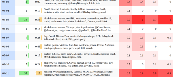
A few years back, I helped a panellist on the Northern Territory’s Scientific Inquiry into Hydraulic Fracturing to analyse concerns about social impacts expressed in more than 600 public submissions. Rather than manually reading every submission to see which ones were relevant, I used a computational technique called probabilistic topic modelling to automatically index the submissions according to the topics they discussed. I was then able to focus my attention on those submissions that discussed social impacts, making the job a whole lot easier than it otherwise would have been. In addition, the topic model helped me to categorise the submissions according to the types of social impacts they discussed, and provided a direct measurement of how much attention each type of impact had received.

This experience proved that computational text analysis methods can indeed be useful for assessing public input to policy processes. However, it was far from perfect case study, as I was operating only on the periphery of the assessment process. The value of computational methods could be even greater if they were incorporated into the process from the outset. In that case, for example, I could have indexed the submissions against topics besides social impacts. As well as making life easier for the panellists responsible for other topics, a more complete topical index would have enabled an easy analysis of which issues were of most interest to each category of stakeholder, or to all submitters taken together.

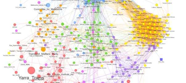
In this post, I want to illustrate how topic modelling and other computational text analysis methods can contribute to the assessment of public submissions to policy issues. I do this by performing a high-level analysis of submissions to the Victorian parliament about a proposal to expand Melbourne’s ‘free tram zone’. I chose this particular inquiry because it has not yet concluded (submissions have closed, but the report is not due until December) and because it received more than 400 hundred submissions, which although perhaps not an overwhelming number, is surely enough to create a sense of foreboding in the person who has to read them all.

This analysis is meant to be demonstrative rather than definitive. The methods I’ve used are experimental and could be refined. More importantly, these methods are not supposed to stand on their own, but rather should be integrated into the rest of the analytical process, which obviously I am not doing, since I do not work for the Victorian Government. In other words, my aim here is not to provide an authoritative take on the content of the submissions, but to demonstrate how certain computational methods could assist the task of analysing these submissions. Continue reading Free as in trams: using text analytics to analyse public submissions

TroveKleaner: a Knime workflow for correcting OCR errors

In a nutshell:

  • I created a Knime workflow — the TroveKleaner — that uses a combination of topic modelling, string matching and other methods to correct OCR errors in large collections of texts. You can download it from the KNIME Hub.
  • It works, but does not correct all errors. It doesn’t even attempt to do so. Instead of examining every word in the text, it builds a dictionary of high-confidence errors and corrections, and uses the dictionary to make substitutions in the text.
  • It’s worth a look if you plan to perform computational analyses on a large collection of error-ridden digitised texts. It may also be of interest if you want to learn about topic modelling, string matching, ngrams, semantic similarity measures, and how all these things can be used in combination.

O-C-aarghh!

This post discusses the second in a series of Knime workflows that I plan to release for the purpose of mining newspaper texts from Trove, that most marvellous collection of historical newspapers and much more maintained by the National Library of Australia. The end-game is to release the whole process for geo-parsing and geovisualisation that I presented in this post on my other blog. But revising those workflows and making them fit for public consumption will be a big job (and not one I get paid for), so I’ll work towards it one step at a time.

Already, I have released the Trove KnewsGetter, which interfaces with the Trove API to allow you to download newspaper texts in bulk. But what do you do with 20,000 newspaper articles from Trove?

Before you even think about how to analyse this data, the first thing you will probably do is cast your eyes over it, just to see what it looks like.

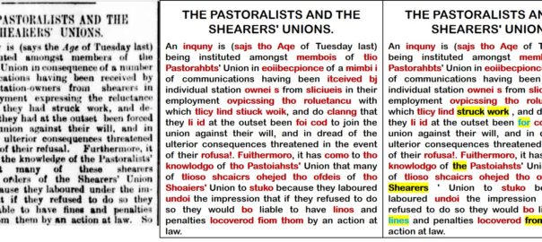
Cue horror.

A typical reaction upon seeing Trove’s OCR-derived text for the first time. Continue reading TroveKleaner: a Knime workflow for correcting OCR errors

Tracking and comparing regional coverage of coal seam gas

In the last post, I started looking at how the level of coverage of specific regions changed over time — an intersection of the Where and When dimensions of the public discourse on coal seam gas. In this post I’ll continue along this line of analysis while also incorporating something from the Who dimension. Specifically, I’ll compare how news and community groups cover specific regions over time.

Regional coverage by news organisations

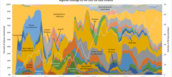
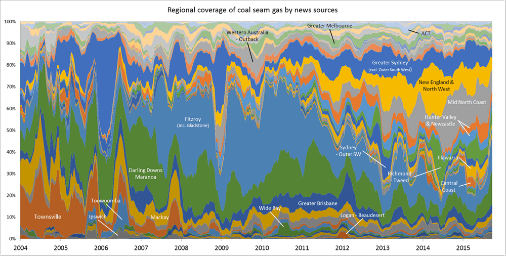
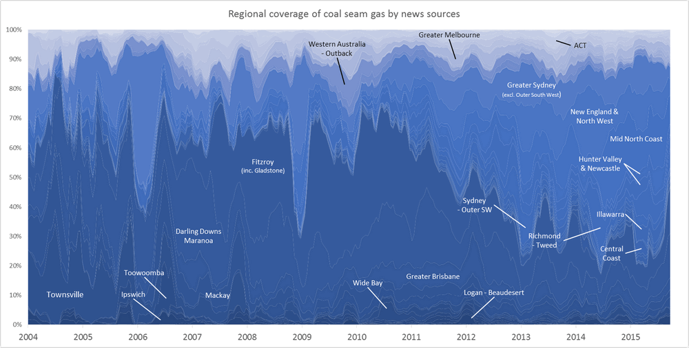
One of the graphs in my last post compared the ratio of coverage of locations in Queensland to that of locations in New South Wales. Figure 1 below takes this a step further, breaking down the data by region as well. What this graph shows is the level of attention given to each region by the news sources in my database (filtered to ensure complete coverage for the period — see the last post) over time. In this case, I have calculated the “level of attention” for a given region by counting the number of times a location within that region appears in the news coverage, and then aggregating these counts within a moving 90-day window. Stacking the tallies to fill a fixed height, as I have done in Figure 1, reveals the relative importance of each region, regardless of how much news is generated overall (to see how the overall volume of coverage changes over time, see the previous post). The geographic boundaries that I am using are (with a few minor changes) the SA4 level boundaries defined by the Australian Bureau of Statistics. You can see these boundaries by poking around on this page of the ABS website.

The regions in Figure 1 are shaded so that you can see the division at the state level. The darker band of blue across the lower half of the graph corresponds with regions in Queensland. The large lighter band above that corresponds with regions in New South Wales. Above that, you can see smaller bands representing Victoria and Western Australia. (The remaining states are there too, but they have received so little coverage that I haven’t bothered to label them.) I have added labels for as many regions as I can without cluttering up the chart.

Figure 1. Coverage of geographic regions in news stories about coal seam gas, measured by the number of times locations from each region are mentioned in news stories within a moving 90-day window. The blue shadings group the regions by state. Hovering over the image shows a colour scheme suited to identifying individual regions. You can see larger versions of these images by clicking here and here.

Continue reading Tracking and comparing regional coverage of coal seam gas