Topic models: a Pandora’s Black Box for social scientists
Probabilistic topic modelling is an improbable gift from the field of machine learning to the social sciences and humanities. Just as social scientists began to confront the avalanche of textual data erupting from the internet, and historians and literary scholars started to wonder what they might do with newly digitised archives of books and newspapers, data scientists unveiled a family of algorithms that could distil huge collections of texts into insightful lists of words, each indexed precisely back to the individual texts, all in less time than it takes to write a job ad for a research assistant. Since David Blei and colleagues published their seminal paper on latent Dirichlet allocation (the most basic and still the most widely used topic modelling technique) in 2003, topic models have been put to use in the analysis of everything from news and social media through to political speeches and 19th century fiction.
Grateful for receiving such a thoughtful gift from a field that had previously expressed little interest or affection, social scientists have returned the favour by uncovering all the ways in which machine learning algorithms can reproduce and reinforce existing biases and inequalities in social systems. While these two fields have remained on speaking terms, it’s fair to say that their relationships status is complicated.
Even topic models turned out to be as much a Pandora’s Box as a silver bullet for social scientists hoping to tame Big Text. In helping to solve one problem, topic models created another. This problem, in a word, is choice. Rather than providing a single, authoritative way in which to interpret and code a given textual dataset, topic models present the user with a landscape of possibilities from which to choose. This landscape is defined in part by the model parameters that the user must set. As well as the number of topics to include in the model, these parameters include values that reflect prior assumptions about how documents and topics are composed (these parameters are known as alpha and beta in LDA). 1 Each unique combination of these parameters will result in a different (even if subtly different) set of topics, which in turn could lead to different analytical pathways and conclusions. To make matters worse, merely varying the ‘random seed’ value that initiates a topic modelling algorithm can lead to substantively different results.
Far from narrowing down the number of possible schemas with which to code and analyse a text, topic models can therefore present the user with a bewildering array of possibilities from which to choose. Rather than lending a stamp of authority or objectivity to a textual analysis, topic models leave social scientists in the familiar position of having to justify the selection of one model of reality over another. But whereas a social scientist would ordinarily be able to explain in detail the logic and assumptions that led them to choose their analytical framework, the average user of a topic model will have only a vague understanding of how their model came into being. Even if the mathematics of topics models are well understood by their creators, topic models will always remain something of a ‘black box’ to many end-users.
This state of affairs is incompatible with any research setting that demands a high degree of rigour, transparency and repeatability in textual analyses. 2 If social scientists are to use topic models in such settings, they need some way to justify their selection of one possible classification scheme over the many others that a topic modelling algorithm could produce, 3 and to account for the analytical opportunities foregone in doing so.
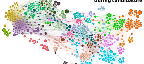
If you’ve ever tried to interpret even a single set of topic model outputs, you’ll know that this is a big ask. Each run of a topic modelling algorithm produces maybe dozens of topics (the exact number is set by the user), each of which in turn consists of dozens (or maybe even hundreds) of relevant words whose collective interpretation constitutes the ‘meaning’ of the topic. Some topics present an obvious interpretation. Some can be interpreted only with the benefit of domain expertise, cross-referencing with original texts, and perhaps even some creative licence. Some topics are distinct in their meaning, while others overlap with each other, or vary only in subtle or mysterious ways. Some topics are just junk.
If making sense of a single topic model 4 is a complex task, comparing one model with another is doubly so. Comparing many models at a time is positively Herculean. How, then, is anyone supposed to compare and evaluate dozens of candidate models sampled from all over the configuration space? Continue reading Qualitative evaluation of topic models: a methodological offering
Notes:
- The generative model of LDA assumes that each document in a collection is generated from a mixture of hidden variables (topics) from which words are selected to populate the document. The number of topics in the model is a parameter that must be set by the user. The proportions by which topics are mixed to create documents, and by which words are mixed to define topics, are presumed to conform to specific distributions which are sampled from the Dirichlet distribution, which is essentially a distribution of distributions. The shape of these two prior distributions is determined by two parameters—often referred to as hyperparameters to distinguish them from the internal components of the model—which are usually denoted as alpha (α) and beta (β). Whereas alpha controls the presumed specificity of documents (a smaller value means that fewer topics are prominent within a document), beta controls the presumed specificity of topics (a smaller value means that fewer words within a topic are strongly weighted). Like the number of topics, these hyperparameters are set by the user, ideally with some regard for the style and composition of the texts being analysed. ↩
- It’s important to recognise that criteria such as transparency and repeatability are not applicable to all textual analysis traditions. Some traditions assume a degree of interpretation and subjectivity that render such criteria all but irrelevant. The probabilistic nature of topic models presents a very different set of challenges and opportunities to such traditions, at least insofar as practitioners are inclined to use them. ↩
- That is, assuming that only one fitted topic model is used in the analysis. Conceivably, an analysis could use and compare several models. ↩
- In this post, as in much of the literature on topic modelling, the term ‘topic model’ may describe one of two things. The more general sense of the term refers to a particular generative model of text, which may or may not be paired with a specific inference algorithm. In this sense, LDA is one example of a topic model, and the structural topic model is another. The second sense of the term refers to the outputs, in the form of term distributions and document allocations, obtained by applying a topic model in the first sense to a particular collection of texts. (These outputs may also be referred to as a ‘fitted topic model’.) The relevant sense of the term will usually be evident from the context in which it is used. ↩