In a nutshell:
- I created a Knime workflow — the TroveKleaner — that uses a combination of topic modelling, string matching and other methods to correct OCR errors in large collections of texts. You can download it from the KNIME Hub.
- It works, but does not correct all errors. It doesn’t even attempt to do so. Instead of examining every word in the text, it builds a dictionary of high-confidence errors and corrections, and uses the dictionary to make substitutions in the text.
- It’s worth a look if you plan to perform computational analyses on a large collection of error-ridden digitised texts. It may also be of interest if you want to learn about topic modelling, string matching, ngrams, semantic similarity measures, and how all these things can be used in combination.
O-C-aarghh!
This post discusses the second in a series of Knime workflows that I plan to release for the purpose of mining newspaper texts from Trove, that most marvellous collection of historical newspapers and much more maintained by the National Library of Australia. The end-game is to release the whole process for geo-parsing and geovisualisation that I presented in this post on my other blog. But revising those workflows and making them fit for public consumption will be a big job (and not one I get paid for), so I’ll work towards it one step at a time.
Already, I have released the Trove KnewsGetter, which interfaces with the Trove API to allow you to download newspaper texts in bulk. But what do you do with 20,000 newspaper articles from Trove?
Before you even think about how to analyse this data, the first thing you will probably do is cast your eyes over it, just to see what it looks like.
Cue horror.

A typical reaction upon seeing Trove’s OCR-derived text for the first time.
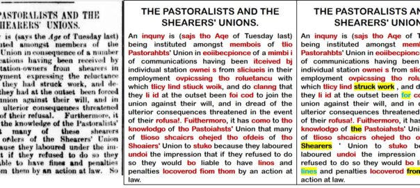
Well what were you expecting, really? Some of the scanned newspapers on Trove are barely readable to the human eye, so it is hardly surprising that the optical character recognition (OCR) system that produced the plain text layer has struggled. Here is a fairly typical example of what this plain text layer looks like, alongside the scanned artefact:
Are all these OCR errors a problem? That depends on what you’re planning to do with the text. Presumably, you won’t be reading it: if you were, you would be better served by the scanned images. More likely, you’ll be mining it using computational techniques such as topic modelling. Or perhaps you’ll be doing something as simple as counting keywords. How will OCR errors affect the results of these methods?
Listed below are the 20 most frequently occurring words (measured by the number of articles in which they occur) in a collection of 20,000 articles published in The Brisbane Courier in the years from 1890 to 1894. Note that prior to tallying the terms, I used a ‘stopword’ list to exclude content-free terms like the and are, and filtered out words shorter than three letters.
tho, Brisbane, south, company, day, Queensland, time, aro, London, government, following, missing, land, havo, house, business, work, own, men, public
There are errors in this list (tho, aro, and havo), but they are of a special kind. They are words that, had they been spelt correctly, would have been identified as stopwords and excluded from the tally. All of the remaining words in the top 20 are spelt correctly. In fact, there are no content-word errors (content-words being those that carry some semantic content, unlike stopwords) all the way down to the 318th most common term, which happens to be paper. At 319th place is Brisbano, which occurs in 2,439 of the 20,000 articles. By way of comparison, Brisbane, its correct form, occurs in 10,894 articles.
So, aside from the problem of stopword errors, lists of frequent terms are basically immune from OCR errors, because the errors occur far less frequently than their correct counterparts.
How does a topic model fare? Here are the top 15 terms of five topics extracted from the same dataset using LDA, a popular topic modelling algorithm.

The first four of these topics are almost pristine: the only error that I can see is loft in Topic 2. To be sure, loft is a valid English word, but its appearance in this topic is likely to be as a mis-spelling of left, which is the second most prominent term in the topic. Furthermore, these topics are highly coherent in terms of the themes or subject matters that they suggest.
The fifth topic is different: it contains almost nothing but stopword errors, along with a few words that are so common (at least in this dataset) or broad in their meaning that they might as well be stopwords. This is an example of what I will call a stopword topic, and is a phenomenon that various other authors have already observed. Topic models are designed to bring together words that frequently co-occur in connection with a given subject, such as horse racing in the case of Topic 1, or shipping arrivals in the case of Topic 2. Whether by accident or design (or a combination of both), it turns out that topic models also bring together words that have no special relationship with any subject matter at all — like stopwords. In cases like the present example, these ‘junk topics’ (as they are sometimes referred to) perform the profoundly useful service of separating unhelpful and content-poor terms from the content-rich terms that we usually care more about.
To summarise, topic models appear to be highly robust to OCR errors. Not only do they separate stopword errors from the substantive topics, they also bundle content-word errors together with their correctly spelt counterparts (like loft and left in Topic 2, above). The latter feature is an inevitable result of how topic models work: since erroneous forms of words will always occur in the same contexts as their correct forms, it follows that errors and their corresponding corrections will be allocated to the same topics. Furthermore, because errors generally occur less often than their correct counterparts (if they don’t, then your text might be beyond help), we can expect errors to have lower weights within a topic than their correct forms.
Topic models therefore perform doubly well in the face of OCR errors. First of all, they produce topics that look clean, because the content-word errors don’t generally feature in the top terms, and the stopword errors get bundled into their own topics. Secondly, topic models can accurately assign topics even to documents that are full of errors, because the modelled topics will generally contain both the correct and erroneous forms of their respective terms.
Good for topic models. But perhaps modelling topics is not what you want to do. Perhaps instead of looking for clusters of words, you want to hunt down and catalogue every occurrence of a particular term. In this case, it might really matter if you miss one out of every five occurrences of the term on account of it being misspelt. Or perhaps you want to apply a named entity recognition algorithm that considers contextual clues like the words before or after a possible name. If these terms are misspelt, the algorithm will ignore or misinterpret them, resulting in names being missed or misclassified.
In other words, if you are interested in describing the needles rather than the haystack, or the trees rather than the forest, then every OCR error is another datapoint lost. Conversely, every correction to these errors is an observation gained.
In my own work with Trove data, my objective was to tag every occurrence of every location that I could map, and tally up the words that most often (or rather, most significantly) occurred with each location. For places that are mentioned rarely (say, in only five articles), every instance counts, and gaining an extra handful of occurrences by correcting OCR errors could mean the difference between having enough information to put it on the map or not. To be sure, I could have produced workable results even without cleaning the text. But I want to squeeze as much as I can out of the data I have. So I decided to have a crack at cleaning the horror-show that is Trove’s OCRd text.
The hunch
Feeling sure that this is a problem that other people must have approached before me, I had a poke around on Google and the academic literature to see what solutions were available.
I didn’t find anything that I was in a position to use. The methods described in research papers typically came with no accompanying code, and in any case I was not keen to spend hours learning to work in Python or whatever language the code would have been in (I was, after all, finishing my PhD at the time as well as embarking on the Trove mapping side-project). Insofar as I could understand how the published methods worked, I wondered about their ability to scale to a collection of tens of thousands of documents, and to work with idiosyncratic language and names. Generally, they seemed to be pitched at correcting individual documents, one word at a time, by using a large reference corpus to build statistics about which words usually follow others.
In any case, I had a hunch that I could at least partly achieve my goal by using tools and techniques that were already within my command. If you’ve been reading this post closely, you might already have an idea of what this hunch was.
The method I developed rests on the following three assumptions:
- LDA will generally allocate OCR errors into the same topics as their correct forms (such as loft and left in the example discussed earlier).
- The correct form of a term will almost always have a higher weight within a topic than its erroneous forms, because the correct form occurs more often than any individual erroneous variant.
- The erroneous form of a term will look very similar to the correct form — that is, it will only differ by one or a few characters.
Given these assumptions, I figured that it should be possible to compile a list of term substitutions that would reliably correct many of the errors in the text. Pairs of terms could be identified as errors and corrections if they (1) appear in the same topic(s), (2) are morphologically similar, and (3) differ substantially in their topic weights (the assumption being that the more highly weighted term is the correct version).
As I will demonstrate shortly, this logic more or less bears out, but only when a couple of other conditions are added. First, the error term must not be a valid English word; and second, the two terms must not be variants of one another, such as singular and plural form, or past and present tense. With these assumptions and conditions in place, it turns out that you can indeed identify a great number of valid error-correction pairs in a large collection of texts.
To be clear, this approach is very different from state-of-the-art approaches to automated OCR correction, which (from what I can gather) examine every likely error and attempt to correct it by analysing the words that come immediately before and after it. My approach instead looks for errors whose correct forms can be reliably predicted from their morphology alone — so, for example, the term Brisbano will in every instance be corrected to Brisbane, regardless of what comes before or after.
This is an inherently limiting approach to correcting OCR errors. Before we even start, we know that this method will not correct every error. Not only is it dependent on the probabilistic whims of a topic model, but it can only fix errors that are not recognised words (so it will in fact treat loft as correct, even if it should be left), and that have only one likely correct form.
Still, something is better than nothing. To be honest, I don’t even know what the next best (or next better) alternative is. I’ve only managed to source one other easily accessible package for this purpose — an experimental Python project called Ochre — and I haven’t gotten around to trying it out. One thing I can say with confidence is that seeing this experiment through has been an enlightening experience. And if you are curious about things such as topic models, string matching, and semantic similarity, there is a good chance that you will find the remainder of this post enlightening as well.
The workflow
As I mentioned upfront, I realised this experimental vision in the form of a Knime workflow, which I’ve named the TroveKleaner (although it will of course work with texts from sources other than Trove). I’ve already written at length about Knime and what it could offer to folk in the digital humanities and computational social sciences. In short, I think it’s an ideal tool for people who are keen to play with data but who are not so keen to invest the many hours it takes to learn to code in R or Python. In addition, Knime workflows can be crafted so that they are highly accessible to other users. Because Knime’s interface is already graphical, with only a small amount of additional effort you can fashion a workflow into something that approaches a primitive user interface. I’ve done my best to construct and document the TroveKleaner so that it can be navigated, used, and customised by users with no coding experience. To use it, all you need to do is point, click, and read instructions. You can download it from the KNIME Hub.
Here is what the top level of the TroveKleaner workflow looks like:
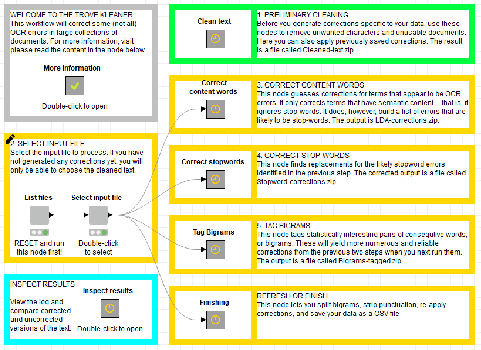
The magic all happens inside the five boxes that are arranged as a column in the middle of the screen. Each of these ‘metanodes’ contains a series of nodes that perform a specific operation on the text, as indicated by their labels and the accompanying annotations. The components of the workflow are separated in this manner so that they can be applied iteratively and in whatever order the user prefers. There are, however, some things that do need to happen before others, as I will explain below.
Input data
Needless to say, prior to running this workflow, you will need to have some text that you want to clean. I have designed the TroveKleaner to work with newspaper data downloaded from Trove with my KnewsGetter workflow. But it should work with data from any source, as long as you name the columns so that they are consistent with the names used by the workflow. Your data will need to be the form of a single CSV file or Knime table.
Perhaps more important than the origin of your data is the amount of it, as this workflow uses methods that work best with large amounts of data. I haven’t tested the limits, but I suspect that your collection would need to contain at least a few thousand documents for the workflow to perform well, and at least several hundred for it to work at all. The upper limit depends only on the level of your patience and the power of your computer.
Preliminary cleaning
This first part of the workflow is like the hair and make-up booth, where your data gets tidied up before stepping onto the main stage. The steps are described in more detail below. Other than the format conversion and the saving of outputs, these steps are optional.
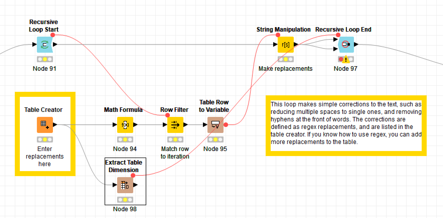
Applying formula-based corrections
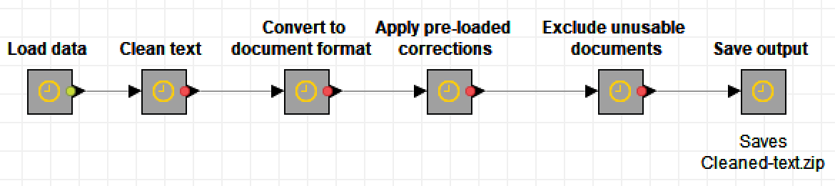
Depending on where your data has come from, it might benefit from some pattern-based corrections to remove things like unwanted hyphens and whitespace characters, along with any characters that might break later parts of the workflow. If you are familiar with regex formulas, you can edit the list of replacements to better suit your own data. This all happens in the ‘Clean text’ metanode, the contents of which look like this:
Tokenising terms
Plain text formats like CSV files store text as strings of characters, which include letters, numbers, punctuation marks and spaces. However, most of the operations in this workflow will work with the text as sequences or ‘bags’ of words or terms. The strings must therefore be converted into tokenised documents in Knime’s native document format.
Applying pre-loaded corrections
While the whole point of the TroveKleaner workflow is to generate and apply corrections that are specific to your data, you might also want to take advantage of corrections that have been extracted from data similar to your own. You can do this within the ‘Apply pre-loaded corrections’ metanode. For demonstration purposes, I have included in the workflow the corrections that I generated from the 82,000 articles published in the Brisbane Courier between 1890 and 1894. These corrections might be useful if you are working with similar data from Trove. Or they might do more harm than good. Don’t say you weren’t warned!
Excluding unusable documents
If you’ve spent any time browsing Trove’s newspapers, you’ll know that some articles, pages, issues, and titles are more readable than others. Some articles look crisp and clear, while others look blurry or smudged. These visual qualities correlate with the quality of the OCR text layer. The best articles have few if any errors, while the worst contain more errors than valid words. Articles fitting the latter description will likely do more harm than good if they are fed to the TroveKleaner workflow.
The ‘Exclude unusable documents’ metanode allows you to filter out any articles in which the relative number of errors exceeds a given threshold. By default, the workflow will exclude articles in which at least a quarter of all unique terms are not in the English dictionary, but you can easily set the threshold to meet your own needs.
Once these steps have been completed, the outputs will be saved as a zip file in a specific location relative to the workflow. The outputs are zipped because otherwise they can become very, very big, due to the way in which Knime saves tokenised documents.
Correcting content-words
Now that the data has been cleansed, the fun can begin. The heart and soul of this workflow lies inside the ‘Correct content words’ metanode:
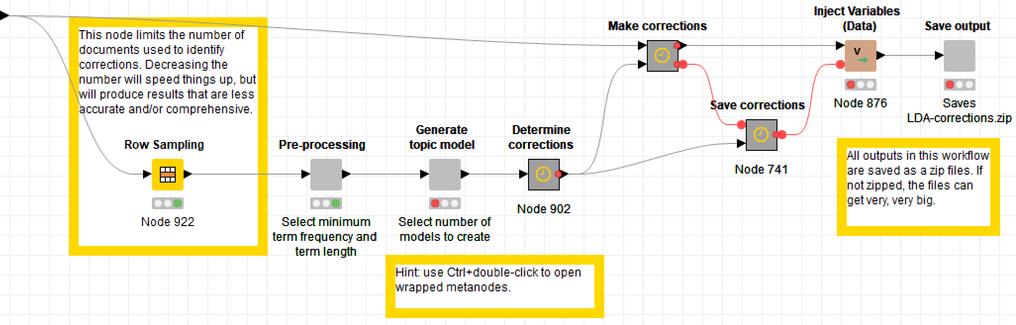
This series of metanodes (the plain grey ones are ‘wrapped’, and can be configured via quickforms) creates a topic model from the input text, extracts pairs of errors and corrections from the topics, and applies these corrections to the input text. In this post, I will describe these steps at a high level and show some example outputs. If you explore the workflow itself, you’ll find annotations describing the steps in much more detail.
All of the outputs that I will present below were produced from a dataset of 82,000 articles published in The Brisbane Courier between 1890 and 1894. While I could have tested this workflow on a much smaller dataset, I wanted to see how it would handle a heavy load. As you can see in the screenshot above, I resorted to sampling the data in order to speed things up. I still applied the corrections to all 82,000 articles, but in each iteration I used a random sample of 20,000 articles to generate the list of corrections. Even then, it took an hour or more to run each iteration of the workflow. (Welcome to the world of data science, where practitioners typically spend around 60% of their time cleaning and organising data, on top of the 19% of time already spent collecting it.)
Pre-processing
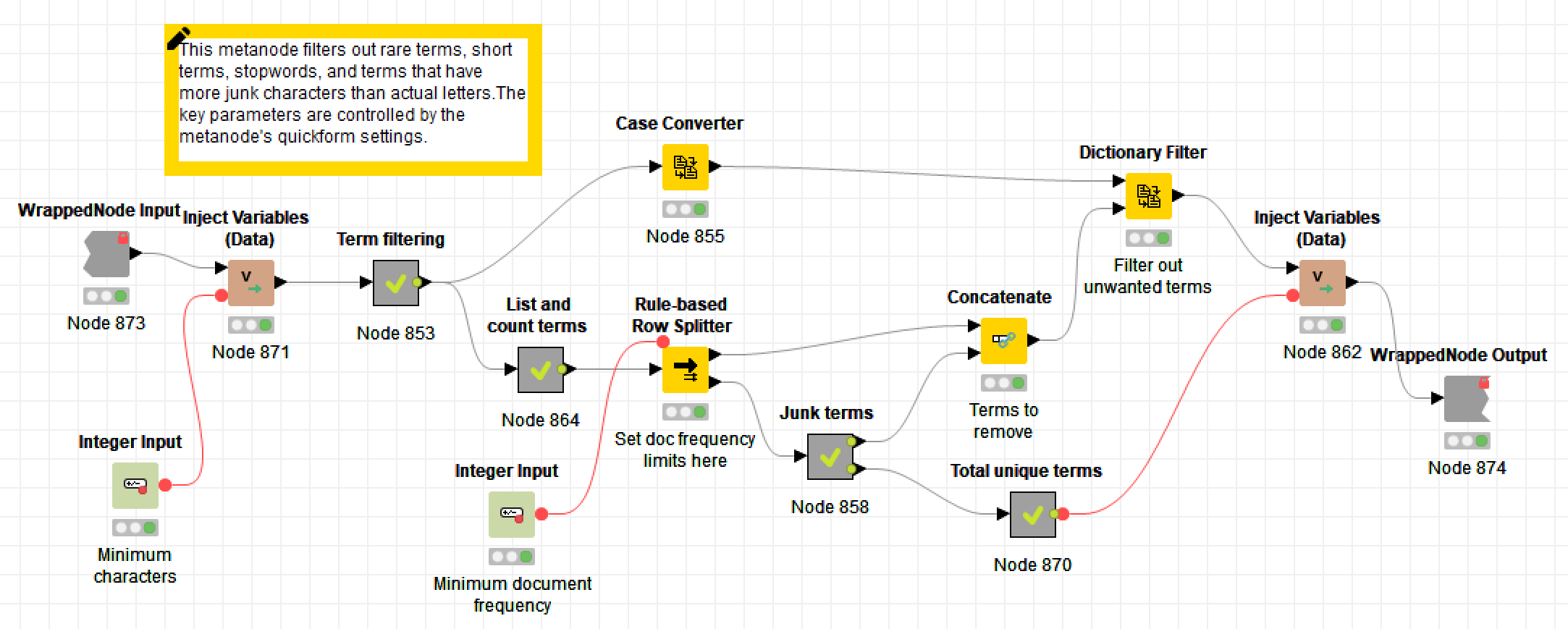
As is customary before creating a topic model, this part of the workflow removes as much unwanted ‘noise’ from the text as possible. This noise includes stopwords, numbers, punctuation, capitalisation, and very short terms.
However, given the aims of the workflow, some of these steps have to be done with a little more care than usual. Numbers and punctuation cannot be removed wholesale, because they may feature in some of the errors that need to be fixed. Brisbane, for example, might be misspelt as 8risbane, or sale might have been twisted into sa/e. On the other hand, terms that comprise more numbers or symbols than letters are likely to be beyond help: perhaps another correction method could fix them, but not this one. Numbers and punctuation are therefore removed via customised rules rather than with Knime’s purpose-built nodes. 1
Short terms are also treated a little differently. Typically, terms that are at least three letters long are retained in a topic model. However, the techniques by which corrections are identified in this workflow do not work well with three-letter words. The lower limit is therefore set at four letters — unless you are just building a list of stopword errors, in which case you should drop it to three.
Finally, terms are excluded if they only appear in a few documents. Doing this can drastically reduce the number of unique terms in the data, thereby speeding up the topic modelling process. However, rare terms may also account for many of the OCR errors the dataset, so omitting them will reduce the number of errors corrected. To deal with this trade-off, I suggest starting with the threshold relatively high, and lowering it in subsequent iterations as the number of unique terms in the data reduces.
Topic modelling
As I mentioned earlier, this workflow employs topic modelling — specifically LDA, which is the only algorithm available in Knime — to cluster OCR errors with their correct forms, with a view to discovering pairs of terms that denote errors and their correct substitutions. What I didn’t explain is why topic modelling is so important in achieving this outcome.
Recall that my method relies on finding pairs of terms that, among other things, look similar to one another. There are well-established methods for finding such pairs, a popular choice being the Levenshtein distance, also called the edit distance because it counts the number of additions, deletions and substitutions needed to transform one string of characters into another. By measuring the edit distance between every pair of terms (that is, every possible pair, not every sequential pair) in a dataset, you can come up with a list of pairs whose members are similar enough to be OCR-induced variants of one another.
However, comparing all pairs of terms in this manner is less than ideal, for two reasons. First, the calculations become exponentially onerous as the number of unique terms in a dataset increases. If your data contained just 10 unique terms, there would 45 possible pairs. In 100 terms, there would be 4,950 pairs. In 10,000 terms — a much more realistic figure if your data contains thousands of documents — there will be 49,995,000 possible pairs. Trust me: calculating the edit distance for this many pairs of terms will take longer than you are willing to wait.
The second problem is that comparing all possible pairs of terms in a dataset is likely to introduce pairings that we don’t want or care about. We really only want to consider pairs of terms that occur in the same contexts, since this is what we expect OCR errors and their correct forms to do.
LDA solves these two problems perfectly, since LDA topics are nothing more and nothing less than clusters of terms that frequently co-occur (even if never all at once). By dividing the terms in a dataset into topics, LDA reduces the number of terms that we need to compare at once, and in doing so it picks exactly the sets of terms that we most want to compare.
There is, however, a complication. Topic models are notoriously bad at making up their minds. Because of their probabilistic and parametric nature, they offer not one but many different ways of carving up the semantic space of a dataset. Tweak a parameter this way or that, or start the algorithm in a different place, and a subtly different set of topics will emerge. Each solution may be valid, but none provides a comprehensive or optimal set of term pairings in which to find corrections.
One antidote to variability is multiplicity. Instead of accepting just one output, we can generate multiple outputs and combine them to ensure that fewer useful solutions are ignored. The TroveKleaner does this in two ways. Firstly, the topic modelling metanode allows you to generate and combine the results of multiple topic models, the parameters of which are partly randomised. 2 Second, the workflow as a whole can (and should) be executed in an iterative fashion, so that the corrected outputs are repeatedly passed back through the error identification process. The iterative nature of the workflow will make more sense as you read on.
Separating stopword topics
Back at the beginning of this post, I showed an example of how LDA tends to bundle stopword errors into their own topics, often along with valid words whose occurrence is not limited to any particular context. Unfortunately, these topics cannot serve as a source of error-correction pairs in the TroveKleaner, because most of the correct stopwords get removed before the topic modelling occurs. 3 These topics are, however, a useful source of stopword errors that can be corrected by other means in a different part of the workflow.
In any case, these stopword topics need to be separated from the other, more substantive topics. There are various ways in which this might be achieved. One logical approach which I did not get around to trying would be to compare the top terms of each topic with those in the stopword list by using the Levenshtein distance. Topics whose terms are highly similar to the stopwords could safely be classified as stopword topics.
Another logical approach would be to measure the coherence of the topics. Coherence in this context means that the terms in a topic are thematically related to one another. In a highly coherent topic, all of the top terms will all clearly relate to a particular theme that features in the text. In an incoherent topic, the terms will have no thematic connection with one another, which is exactly the case with stopwords. This type of coherence has been successfully approximated with a measure called pointwise mutual information, or PMI, which essentially measures the significance of two terms co-occurring, given their overall frequencies in a dataset.
It turns out that most stopword topics do indeed have low PMI values. 4 However, it also turns out that some stopword topics have very high PMI values. As far as I can tell, these are topics whose terms all result from a particular type of OCR error, perhaps brought about by a specific kind of visual blur or artefact that occurs in some documents and not others. Because these specific errors all frequently occur together, the resulting topic is highly coherent. This is a good reminder that LDA does not just cluster words around topics in the usual sense — it clusters them around whatever drivers of structure there might be, whether authors, writing style, or image artefacts.
Another problem with calculating PMI is that it adds considerable computational load to the workflow. Ultimately, I managed to achieve satisfactory results without it, by applying some simple rules and metrics of my own devising. For example, it turns out that the top terms of stopword topics tend to be relatively short, fairly uniform in length, and include relatively few unique characters. Another class of stopword topics in my data contained mostly terms that started with ‘x’, such as xvith and xvill. These sorts of rules do not perform perfectly every time, but they seem to work well enough for the purposes of the workflow. Depending on the nature of your data, it is possible that other metrics such as PMI will need to be added to produce adequate results.
Once the stopword topics are separated, some of their terms are saved for later analysis. The terms that are not saved are those that are valid English words or whose overall occurrence is below a threshold value. Rarer terms are excluded because the methods used to correct these terms later on are unlikely to work without a critical mass of occurrences.
Finding the corrections
So, we have our topics. How do we now go about finding pairs of terms that could be used reliably to correct OCR errors? This is by far the most complex part of the worklfow, so sit tight.
The first step, as earlier parts of this post have already alluded to, is to calculate the edit distance between all pairs of terms in each topic. If you keep the number of terms in each topic to within a couple of thousand, this does not take inordinately long (though typically still long enough to make a cup of tea). We can then exclude most of the resulting pairs, as we only want those whose similarity is above a reasonable threshold.
The next step is to compare the topic weights (essentially the overall term frequencies) of the terms in each pair. The workflow calculates a ratio from these values, and also assumes that the more highly weighted term in each pair is the correct form, while the less prominent term is the error. In performing this step, the workflow averages the weights of terms that appear in multiple topics. 5
The third step is to exclude pairs in which the error term is a valid English word, or in which the two terms are valid tense variants (such as plurals or past tense) of one another. Excluding English words from the errors means that some errors — such as loft and left in the earlier example — will go uncorrected, but distinguishing valid words that are errors from those that are not is a challenge that I did not even try to address. 6 To identify tense variants, I used a method that I have previously developed for stemming terms in a way that is both gentle and dataset-specific. Essentially, this method works by searching for pairs of terms in the data that match a list of formulas that capture common tense variations, such as plurals ending in ‘s’ or past-tense forms ending in ‘ed’. If one variant occurs much more frequently than the other, then it will replace the less common variant throughout the text.
What remains from the preceding steps is a set of candidate corrections, most of which will not be valid. To sort the wheat from the chaff, I developed a composite score that combines several pieces of evidence that a pair of terms is really a valid error and correction. These pieces of evidence are:
- the weight ratio (the bigger the better, as errors tend to occur much less often than the correct words)
- the edit distance (terms that are more similar are more likely to be variants of one another)
- the ratio of term lengths (this is captured to some extent by the edit distance, but is a useful differentiator nonetheless)
- the overall log weight of the error (this is perhaps the most dubious of the values, but helps because in general, errors have lower weights than corrections)
To calculate the composite score, I first normalised these values, then weighted them according to their importance, and then normalised the score obtained by adding them together. I’m not going to lie: this score is a complete hack. It works, but I have little doubt that it could be formulated in a more rational way.
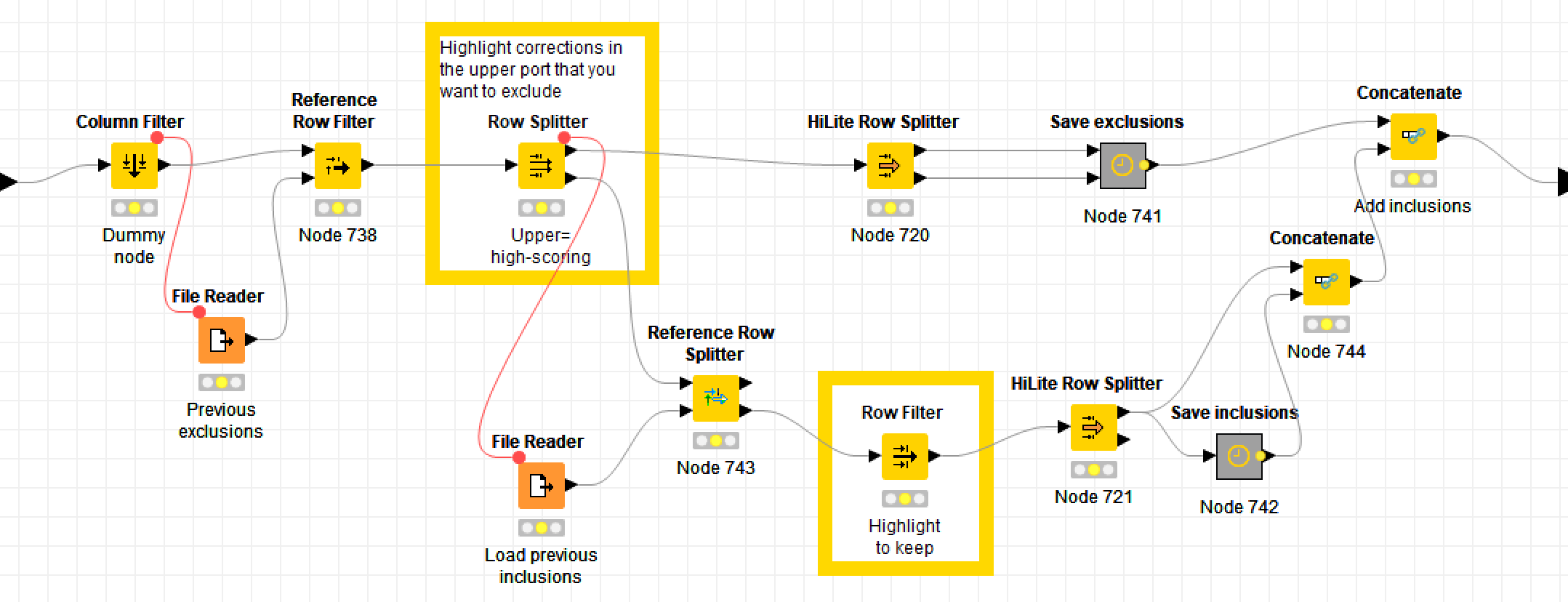
Having scored the pairs, I found a threshold value above which, in every instance, nearly all of the pairs were valid corrections. (In case you’re wondering, the magic number is 0.7, though sometimes it needs to be raised to 0.72 for the first iteration.) The workflow excludes all pairs below this threshold, but allows you to manually add and remove specific pairs, and applies these interventions to all subsequent iterations. Of course, you can also adjust the threshold itself.
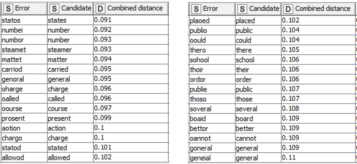
Drawing on the combined results of two topic models, derived from a sample of 20,000 documents from my dataset, this process yielded 8,556 corrections, the top 63 of which are shown below.
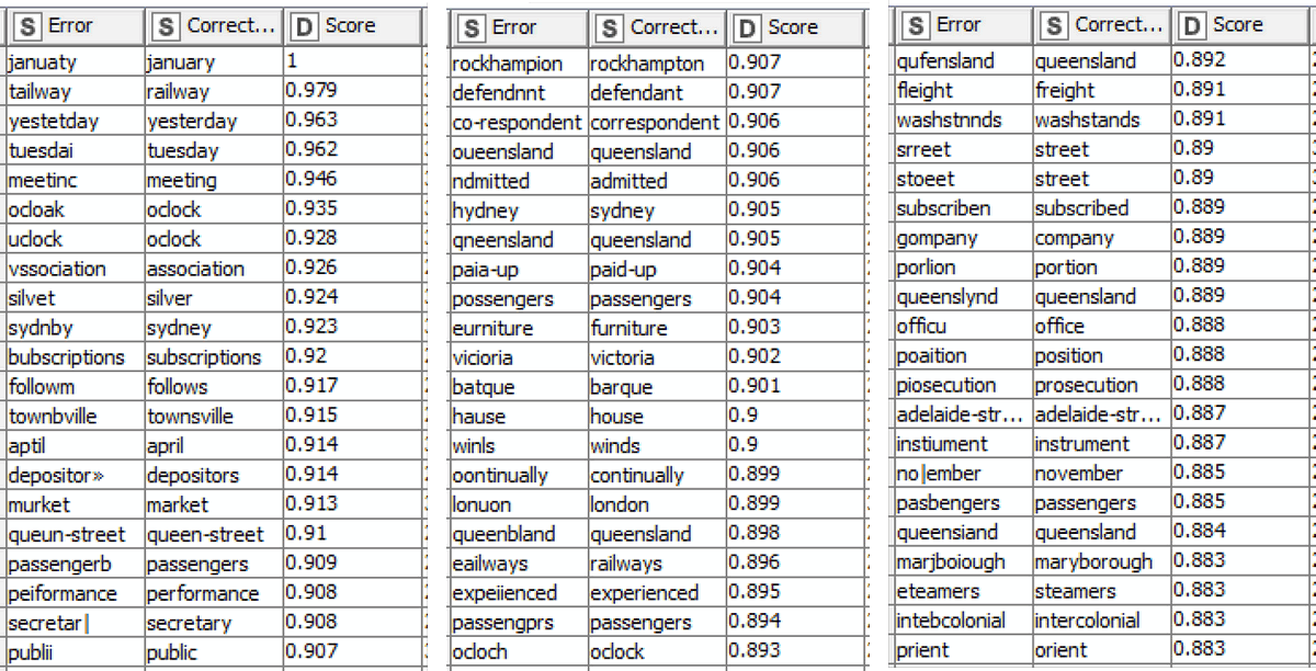
To be sure, these are the very best of the outputs rather than a representative sample. But they are sufficient to illustrate the nature of the corrections that the TroveKleaner discovers. A different appreciation of these outputs can be gained by looking at all of the corrections that are discovered for a single term, in this case Queensland:
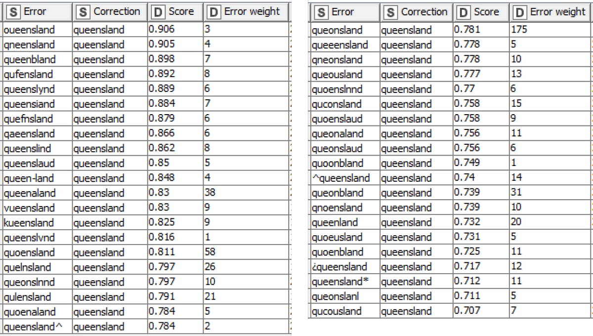
In this example I’ve also included the error weight, which corresponds roughly with the overall frequency of the error in the 20,000 sampled documents. Given that Queensland occurs 29,225 times in the same sample, it’s fair to say that most of these errors are very rare in comparison with their correct form.
When looking at these examples, keep in mind that all terms were converted to lowercase before the topic modelling process, so some of these pairs actually reflect corrections that apply to capitalised terms. This explains recurring substitutions such as ‘b’ to ‘s’ (as in bubscriptions to subscriptions) and ‘f’ to ‘e’ (as in eurniture to furniture), as these letters resemble each other much more closely in upper case. In the next section, I’ll explain how different capitalisations are considered when the corrections are applied to the text.
The sad thing about this method is that many more valid corrections end up getting excluded because they lie beneath the threshold value of the composite score. This is an inevitable outcome of setting the threshold high enough to obtain high-quality results. And while you could manually comb through the rejects to retrieve the valid corrections, it’s very possible that there are better ways you could use your time. A better approach would be to take some consolation in knowing that some of those valid corrections will score higher in a subsequent iteration. And if you think you can improve the quality of the score upon which the threshold is based, please be my guest!
Applying the corrections
Finally, it’s time to apply the corrections to the original data! This should be the simple part, and in relative terms it is, but it’s not as straightforward as simply finding and replacing all of the terms on the list. The first issue to contend with is that Knime’s Dictionary Replacer node does not give you the option of ignoring case. Thankfully, the Dictionary Tagger node does. So before making the replacements, the workflow tags every occurrence of each error term and compiles a list of case variants for each. (Unfortunately, this step can take a long time if your dataset is large.) It then uses a set of rules to come up with an appropriate capitalisation for the correction of each of these variants.
The second complication is that not all of the corrections result in valid words. Some of them only produce a result that is closer to the correct version than the original error. Brishano, for example, might get corrected to Brisbano. However, in many cases the correction list also contains the substitution that is needed to turn the the part-correction into the correct term — that is, to turn Brisbano into Brisbane. In order to join these chains of corrections, the TroveKleaner makes the corrections in several iterations, each time applying another step of the chain.
Once the corrections are made, the workflow saves the results as a new zip file, or overwrites the previous output from this process if one exists. Along the way, the workflow also saves the results of the process into a log file through which you can track the results of each iteration that you perform.
Correcting stopwords
Recall that during the process of correcting the content words, the TroveKleaner saved a list of stopword errors to be dealt with separately. Predictably enough, this separate process happens in the metanode labelled ‘Correct stopwords’.
Like the method for correcting content words, the stopword correction process also combines string similarities with contextual information to compile a list of reliable substitutions. But whereas the content word corrections used semantic context to narrow the field, the stopword corrections draw on what you could call syntactic or grammatical context — that is, the words that commonly appear immediately before and after the term.
To be more specific, TroveKleaner accepts a term as a correction for a given stopword error if:
- the correction occurs much more frequently than the error
- the correction is morphologically similar to the error, and
- the correction appears before and after similar words as the error.
The sequence of metanodes shown below outlines the process by which this is achieved.
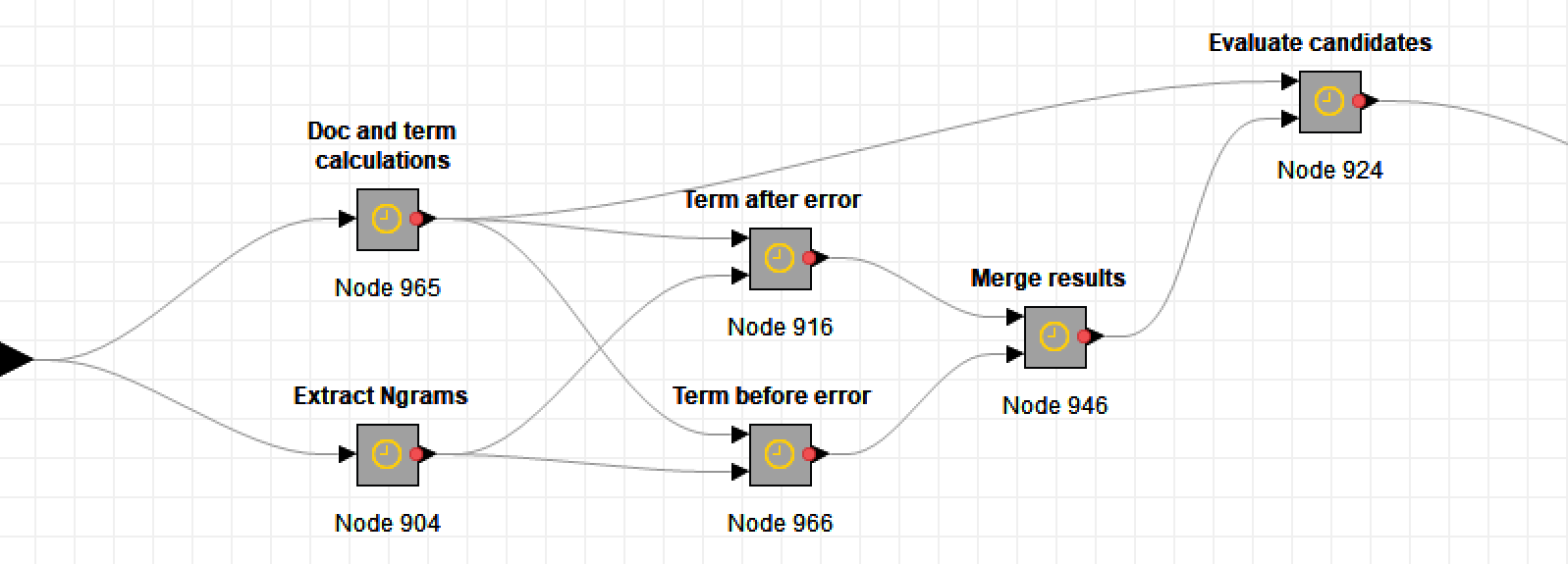
First, the workflow generates a list of all bigrams — that is, sequences of two words — in the dataset (or a sample thereof). It also tallies the number of documents in which each bigram and each individual term (or unigram) occurs.
Then, for every stopword error, and for every valid word that looks similar to the error (as determined by the edit distance), the TroveKleaner trawls through the bigrams to find the words that most frequently occur immediately before and after it in the text.
The workflow then compares the neighbours of each error with those of its candidate corrections. It does this by calculating the cosine distance between pairs of vectors representing the frequencies with which neighbouring terms follow or precede the error and candidate. If an error and candidate have similar neighbours, the cosine distance between them will be small. This all happens in the following sequence of metanodes:
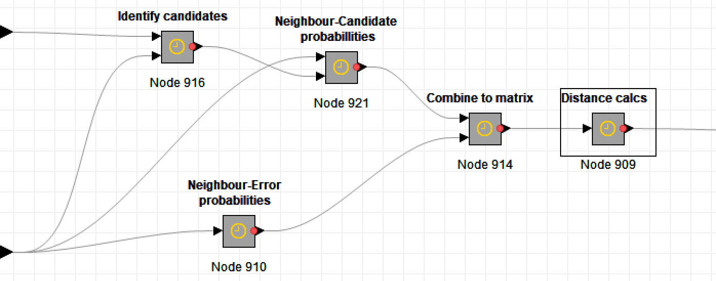
Finally, the workflow builds a composite score combining the various distances and term ratios for each pair, and excludes all but the most promising by way of a threshold. Here is a sample of the resulting corrections, along with their composite scores (smaller scores denote better matches):
These corrections are then applied to the text and the output saved as a new zip file. You could now pass this output straight back into the content word correction process, but if you’re feeling adventurous, there is one more step you should try first.
Better with bigrams
If you look back through the examples shown so far, you’ll notice that all of the terms listed are single words, or unigrams. In natural language, however, some words or names are strung together so frequently that it makes sense to treat them as single units. Two-word sequences of this nature are called bigrams. The reason why the TroveKleaner includes a bigram tagging feature is that bigrams can increase both the number and the quality of corrections that the TroveKleaner discovers.
Bigrams are helpful in this context because they are more distinctive than unigrams. In general, the longer a word, the more robust its identity in the face of spelling corruptions. For example, if you change a random letter in the word correspondent, there will remain little doubt as to what the original word was. But if you do the same to a short word like take, there may be no way for someone to guess the original term, at least without contextual information. Indeed, the new word might not even look like an error. This is why the TroveKleaner struggles with short words.
Put simply, because bigrams are longer than unigrams, they can be more reliably processed by the TroveKleaner. This opens up opportunities for words that would otherwise have been ignored to be corrected, at least when they appear as part of a tagged bigram. In particular, bigrams allow for the correction of short stopwords, as you can see in these stopword corrections, which were generated after bigrams were tagged:
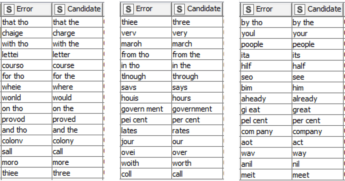
Admittedly, nearly all of the two-word corrections in this example merely change tho to the, but you get the idea. Note also that there are instances in which a bigram is changed into a single word, such as govern ment to government and com pany to company. These instances show that in some cases at least, the TroveKleaner can correct spacing errors as well as spelling errors. And lastly, it’s worth noting that there are a few likely unwanted pairings in this bunch. Before applying these corrections, I would remove jour to our and anil to nil.
Naturally, tagging bigrams comes at a cost — namely, that it increases the number of unique terms in the dataset, which in turn slows down topic modelling and other important processes in the workflow. So you need to be strategic about how many bigrams to tag, and which ones they are. The TroveKleaner prioritises the discovered bigrams by considering both their overall frequency and their pointwise mutual information values, the latter of which indicates how surprised or interested we should be to find two terms together, given their overall frequencies. The thresholds are yours to fiddle with. In doing so, just be careful not to add too many new terms to your data.
If at any point you want to dissolve your tagged bigrams and return to using only unigrams, you can do this with the ‘Split bigrams’ function, which lives within the ‘Finishing’ metanode.
O-C-aahhh?
The examples I’ve shown so far should be enough to convince you that on some level at least, the TroveKleaner does what it is supposed to do. I can promise that it will reduce the number of OCR errors in a large collection of documents such as the newspaper articles on Trove.
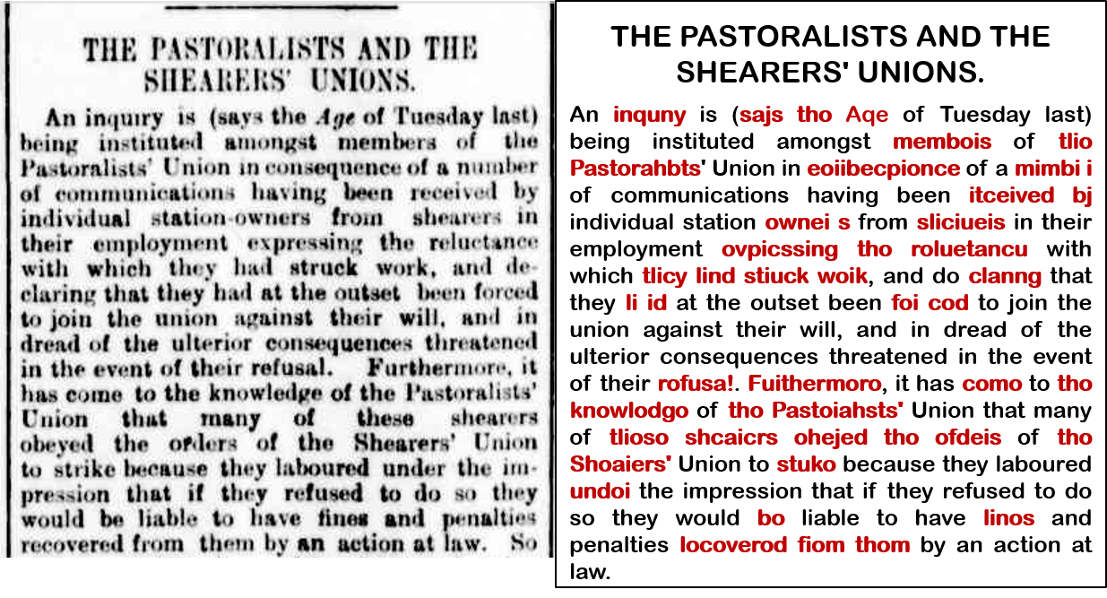
Will it make enough corrections to be worth your while? That depends on what you’re trying to achieve. If you are hoping to turn Trove’s OCR text into something that doesn’t look like it was produced by a blind, intoxicated, fat-fingered typist, then the TroveKleaner may disappoint you. Take a look at the comparison below of an article (the same one as was shown at the beginning of this post) before and after it has gone through several iterations of corrections. I’ve highlighted the terms that have changed in the corrected version.
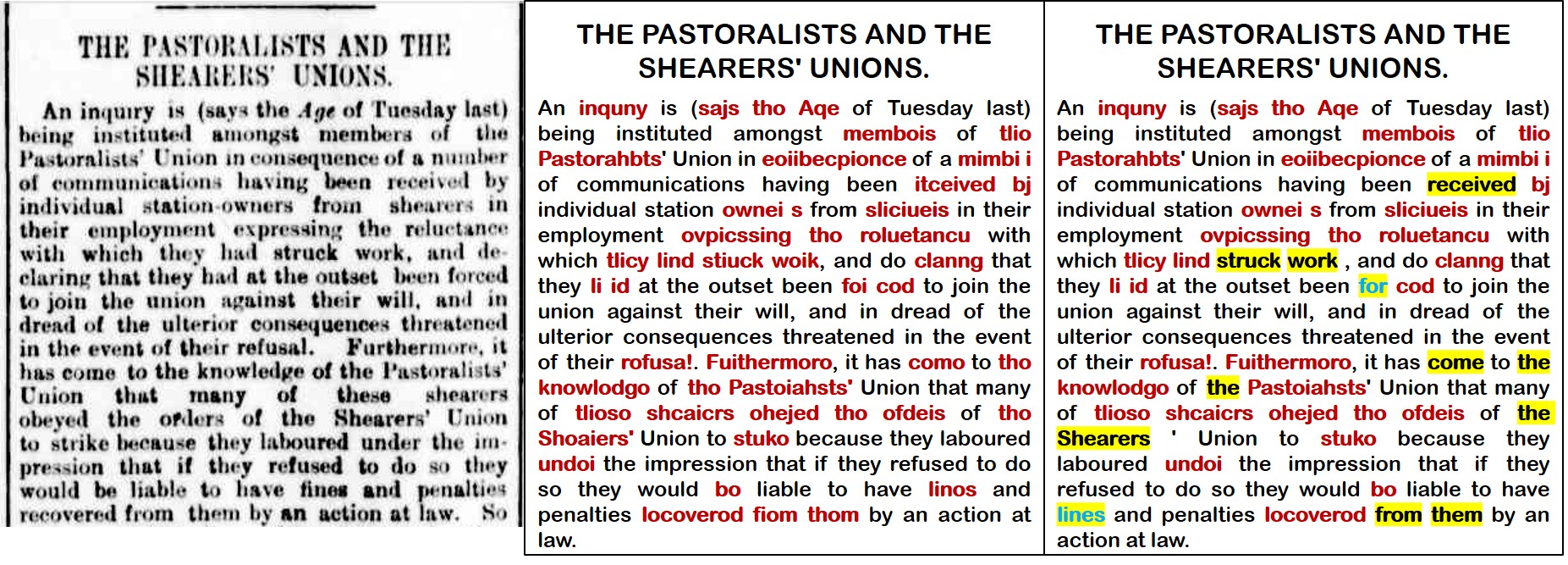
In the 11 iterations of corrections that this article passed through, the TroveKleaner discovered and applied no fewer than 71,654 unique corrections. And yet, when you look at an individual article like this one, it’s clear that these corrections have barely made a dent on the overall number of errors. A few errors have been corrected (most of them stopwords), but many more remain.
Quantifying the number of errors in the data is difficult without a comprehensive list of every correct term (that is, names as well as words), but we can get a rough idea by counting the percentage of terms in each document that do not appear in an English dictionary. Over the course of the ten iterations of corrections, this figure, when averaged across all documents, fell from just above 29% to just below 27%. In other words, about a quarter of all the terms in my data are still errors, even after a day of working my laptop so hard I thought it might melt down.
This is not to say that the TroveKleaner can’t do better. If you felt so inclined, you could keep running further iterations and discovering new corrections. As the first plot below shows, the number of new corrections tends to reduce with each iteration, but increases (along with the processing time) as you admit more terms into the topic model (the number of terms is controlled by the minimum document frequency). However, the second plot shows that the actual number of corrections made in each iteration plummets after the first couple of iterations and then remains more or less flat. This is because the errors corrected in the first few iterations are on average much more common than those in the later iterations.
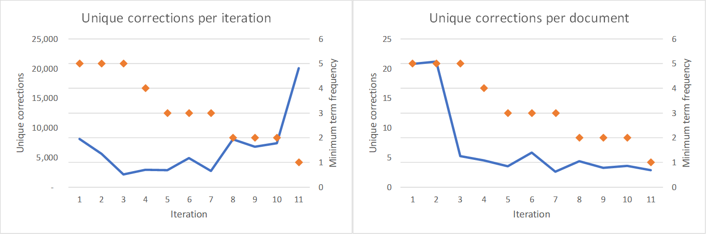
I take these results to be evidence that a large number of the errors in Trove are rarities, or even one-offs. This is unfortunate, because these are the errors that the TroveKleaner is least well equipped to find. Not only does the computation take longer when rare terms are included, but the the quality of results is also likely to decline. Remember that topic models work by grouping terms that regularly occur together. If a term occurs only once or twice, there is very little information that a topic model can use to determine which other terms it belongs with. Consequently, the TroveKleaner might never match the rarest errors with their correct forms.
In other words, the TroveKleaner will not get you all the way from OC-aargh! to OC-aahh. But it will help. Even if individual documents do not look much better, there is something to be said for knowing that the dataset as a whole is healthier. Exactly how this improved health will manifest in your analytical results is hard to say. But if garbage in equals garbage out, then it seems fair to say that the TroveKleaner will help your results to stink a little bit less than they otherwise would. And who knows, if your analysis depends heavily on certain terms that the TroveKleaner has managed to correct, then the payoff could be considerable.
Besides the certainty that the TroveKleaner will correct a percentage of errors, I can also guarantee that it will make some mistakes, especially if the user does not review the corrections before applying them. No OCR correction method is foolproof, and this one is perhaps more liable than most to produce some creative results. So please, use it with care.
The monster
I produced the first version of this workflow last year, during an improbably productive period while finishing my PhD. When I dusted it off a few months ago, I had hoped to pump out a revised and share-worthy version within the space of a few weeks. Before long, the TroveKleaner turned into an evening-stealing, weekend-haunting, time-sucking monster, which has had considerably less time to steal since I started my first post-PhD job. 7
Now that this monster is out in the open, I have to admit that its teeth aren’t even very sharp, and its appetite for fixing errors is not as voracious as I had hoped. As an experiment and a learning experience, it has been successful. As a solution to Trove’s OCR problems, it is only partial. But perhaps it could yet be part of whatever the best solution proves to be. From what I can gather from my (admittedly cursory) review of academic literature, this workflow departs from many other OCR correction approaches in that it draws on nothing except the input data itself to build a dictionary of corrections. 8 This bootstrapping approach obviously carries limitations, but it also has advantages — most notably, it is able to discover corrections for words and names that appear in the collection but not in standard dictionaries. Perhaps this capability could be fruitfully combined (if it hasn’t already) with more more conventional OCR correction approaches.
If you do get any value out of this workflow, I’d love to know. I’d be particularly interested to hear from anyone who is actually across the state of the art in managing OCR errors in archival texts. If it turns out that something I’ve presented here is genuinely new and useful, perhaps you’d like to help me write a paper. On the other hand, if you think I’ve wasted my time, feel free to tell me that too!
Having cut this monster loose, I do have plans to start feeding another one. I still hope to revise the remainder of the workflows with which I have geoparsed and geovisualised Trove newspapers. Next on the list is the geoparser, which, like the TroveKleaner, also employs LDA in a creative way. Expect it later rather than sooner.
Notes:
- As an aside, I should mention that if you plan to remove punctuation from your data altogether — that is, if your analyses all work with a bag-of-words model — then you should consider doing this before making corrections with the TroveKleaner. I’ve noticed in the past that Knime does not always tokenise terms optimally, leaving some terms with punctuation characters attached. Unless you strip out all punctuation before making the corrections, these poorly tokenised terms will not get corrected. ↩
- The alpha value is randomised between 0.03 and and 0.3, while the beta is held steady at 0.01. Large beta values result in topics defined by a greater number of terms, thus slowing down the pairwise comparisons that are performed downstream. The number of topics defaults to 100, but because this also affects the number of terms per topic, you will probably need to adjust it depending on the number of documents being fed to the topic model. The seed is also randomised. ↩
- You could run the topic model with the stopwords included. This tends to result in a messy topic model, but perhaps it could be made to work within the context of the TroveKleaner. ↩
- I should note that David Mimno et al (2011). proposed a similar but apparently better metric than PMI for this purpose, which I have not yet tried. ↩
- I’ve found that doing this delivers the best results, but in theory, there is a good case for keeping a separate set of corrections for every topic. This way, the corrections could be applied only to documents that contain the relevant topics, potentially making the corrections more targeted and reliable. I’ll leave this for someone else to explore. ↩
- If I were to go down this road, I would almost certainly start by retaining topic-specific corrections, as discussed in the previous footnote. ↩
- I’m now working at RMIT University in Melbourne as a researcher on the Future Fuels CRC, which is paving the way for the adoption of hydrogen as an energy carrier and natural gas substitute in Australia. It’s certainly a step up from working on coal seam gas. ↩
- In relation to the TroveKleaner’s use of LDA, there are some published examples where LDA has been used to narrow the range of relevant corrections that are invoked from a dictionary, or by other methods – for example, Wick et al. (2007), Farooq et al. (2009), and Hassan et al. (2011). But I’ve not seen any approaches in which LDA is aprimary vehicle for discovering errors and corrections in the first instance. ↩