This post describes the motivation for the TextKleaner workflow and provides instructions on how to use it. You can obtain the TextKleaner workflow from the KNIME Hub.

Confronting the first law of text analytics

The computational analysis of text — or text analytics for short — is a field that has come into its own in recent years. While computational tools for analysing text have been around for decades — the first notable example being The General Inquirer, developed in the 1960s — the need for such tools has become greater as the amount of textual data that permeates everyday life has increased. Websites, social media and other digital communication technologies have created vast and ever-expanding repositories of text, recording all kinds of human interactions. Meanwhile, more and more texts from previous eras are finding their way into digital form. While all kinds of scholarly, commercial and creative rewards await those who can make sense of this wealth of data, its sheer volume means that it cannot be comprehended in the old fashioned way (otherwise known as reading). Just as computers are largely responsible for generating and transmitting this data, they are indispensable for managing and understanding it.

Thankfully, computers and the people who program them have both risen to the challenge of grappling with Big Text. As computers have become more and more powerful, the ways in which we use them have become more and more sophisticated. No longer a synonym for glorified word counting, computational text analysis now includes or intersects with fields such as natural language processing (NLP), machine learning and artificial intelligence. Simple formulas that compare word frequencies now work alongside complex algorithms that parse sentences, recognise names, detect sentiments, classify topics, and even compose original texts.

Such technologies are not the sole domain of tech giants and elite scientists, even if they do sit at the core of digital mega-infrastructures such as Google’s search engine or Amazon’s hivemind of personal assistants. Many of them are available as free or open-source software libraries, accessible to anyone with a well-specced laptop and a basic competence in computer science.

And yet, no matter how powerful and accessible these tools are, they have not altered a fact that, in my opinion, could be enshrined as the first law of text analytics — namely, that analysing text with computers is really hard.

To be sure, all kinds of statistical analysis are hard to some degree, and most require  considerable expertise to be done correctly. But computational text analysis is hard in some unique and special ways, many of which stem from the tension inherent in trying to quantify and rationalise something as irreducibly complex as human language and communication.

For a start, natural language, which data scientists often refer to as ‘unstructured text’, is an inherently messy form of data. Even before you consider what individual words mean, your computer can have a hard time just figuring out what the individual words are. Where a human looks at a text and sees discrete words separated by spaces and punctuation marks, a computer sees an unbroken string of characters, some of which happen to be letters, and some of which happen to be spaces and other characters. You would think, by now, we would have a universal and fool-proof system for converting strings of characters into discrete words, or tokens. But, as anyone who starts getting their hands dirty with text analytics soon discovers, we do not.

To see why, consider these examples. What we humans see as a space might in fact be a line break or a non-breaking space character, both of which may or may not be parsed differently from an ordinary space character. Where we see an apostrophe or inverted comma, the computer might see any one of several different characters that sometimes get used for the same job. Speaking of inverted commas, how is the computer supposed to know whether you want to tokenise Bob’s as two tokens (Bob and s, or maybe ‘s) or one? Do you even know which you would prefer? What about words joined by backslashes like him/her or either/or? Are they one word each, or two? What about hyphenated words? And so on.

Once the words in a text have been demarcated, the really hard part begins. Computers are really good at counting things, but what, exactly, do you want to count in a textual analysis? Naively, you might think that the most frequently used words will be the most important — until you realise that the most frequent words in just about any English text are function words like the, be, to, of, and and, which on their own are uninformative. So maybe you want to ignore or remove these function words and only count the others. But where do you draw the line? Predefined ‘stopword lists’ can make this choice for you, but if used uncritically could result in meaningful terms being excluded from your analysis.

Suppose you remove all the uninformative words and just count the rest. What more could go wrong? Lots! For a start, words can have different meanings depending on their context. Does the word bark refer to dogs or to trees?  Is bear an animal or a verb? Even if a word has only a single definition, sarcasm can invert its meaning entirely, and is notoriously difficult to detect in a programmable way. Does heat have the same meaning on its own as it does when preceded by on? If not, perhaps we should tag on heat as a single term — in which case, I hope you haven’t already gone ahead and removed all those stop words! Is Green a colour, a political denomination or a person? If it is the latter, is it preceded by a first name that we should really join it to for counting purposes? And so on.

Such considerations may lead you to realise that you don’t want to count individual words so much as more complex or abstract things such as names, concepts or topics. There are tools that help you do just this–but they are far from silver bullets. A named entity tagger, such as the one created by the very clever folk at the Stanford Natural Language Processing Group, will do a pretty good job of detecting and discriminating between the names of people, places and organisations; but almost invariably, it will miss or mis-classify some or many of the names in your text. Meanwhile, probabilistic topic models such as LDA go a long way to solving the ‘context problem’ by counting words not on their own but as members of semantically coherent groups of words, enabling us to know, for example, when the word bark refers to trees and when it refers to dogs. But, as I have written previously, topic models can raise as many questions as they answer, and their use in some contexts reamains controversial.

And what about variations of words such as plurals and past tenses? We might agree to count cat and cats as the same word, but what about tense and tenses, or time and times? What about different capitalisation of the same word? Words that are not names can all be converted to lowercase, but what about names that are formatted in ALL CAPS: do we need to convert them to title case so that they are counted with other instances? And do we need a special rule for those pesky Dutch surnames that start with a lowercase d? And what if some uppercase terms are actually acronyms, and we want to preserve them as such?  Or what if…

And so on. You get the idea. There’s no way around it: for various reasons, analysing text with computers is just really hard. Language and communication do not give themselves up easily to quantification. Nor, for that matter, do they invite easy classification, throwing up one fuzzy boundary after another. For every rule, there are exceptions. For every model, there is a disclaimer. For every simplification, an argument to be had. For every clever trick, there is a situation where it fails spectacularly, or — even worse — so quietly and insidiously that you don’t even notice until you’re just about to go home for the day.

Using KNIME for text analysis

Another way of stating the first law of text analytics is that if it’s not not really hard, you’re probably not doing it right. Indeed, the difficulties and complexities involved can make text analytics outright confronting, especially to the uninitiated, and even more especially to anyone who lacks fluency in coding languages such as R or Python, in which most of the available tools for doing it are written.

My own journey through text analytics started several years ago with my PhD, which ended up being about methodological and conceptual challenges associated with using topic models in social science. Since then, I’ve explored and applied various computational techniques in analyses (some paid, some recreational) of texts including contemporary news, historical newspapers, public submissions to government inquires, and social media content.

One way in which my journey has differed from that of most text analytics practitioners is that it has been enabled not by R or Python, but by a piece of software called KNIME. I’ve already written at length about Knime (with apologies to its developers, I prefer to capitalise it as an ordinary name) and its potential utility for researchers in computational science and digital humanities, so I won’t say much more about it here. The bottom line is that Knime enables you to do much of what you might otherwise do with R or Python, but without the burden of learning how to code at the same time. Instead of requiring precisely formulated code as its input, Knime provides a graphical interface in which you can construct analytical workflows with the help of an extensive repository of ‘nodes’ that perform discrete functions and that can be configured through point-and-click menus. The workflows can be very simple or highly sophisticated, and if constructed thoughtfully can be used and adapted by other users with no coding experience. Like R or Python, the Knime analytics platform is open-source (although it is hitched to an enterprise server product), and draws on software libraries from a variety of other sources. It even allows for the embedded use of R or Python to perform any tasks that cannot be done natively.

Knime’s node repository includes a solid collection of text processing functions, ranging from simple ‘preprocessing’ tasks such as stemming and stopword removal, through to advanced tasks such as named entity tagging and topic modelling. Many of the text processing nodes draw on widely used libraries such as CoreNLP, OpenNLP, and (for topic modelling), MALLET. Just as importantly, Knime’s more general functionality, which includes various kinds of clustering and distance calculations in addition to basic math operations and string manipulations, allows you to weave the text processing nodes into more powerful, task-specific workflows.

Creating such workflows is exactly what I have been doing for several years now. As I have found myself performing certain tasks repeatedly across different jobs, and as I have come to understand the limitations and possibilities both of Knime’s text processing nodes and of the functions they perform, I have gradually built my own customised suite of text processing functions. And finally, I have refined them to the point where I am ready to share many of these functions in an integrated workflow. Behold: the TextKleaner!

Overview of the TextKleaner

As you can probably guess from its name, the TextKleaner is not supposed to be a one-stop-shop for all your text analysis needs. Rather, its purpose is to clean and enrich your data in preparation for a computational analysis. This phase of data preparation is commonly called text preprocessing, as it covers all the things you have to do before you perform your analysis. As you can gauge from the introduction above, text preprocessing is a task that can be every bit as difficult and complex as the analysis itself. Furthermore, decisions you make in preprocessing your data can have a real impact on the results of your analysis.

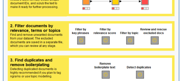
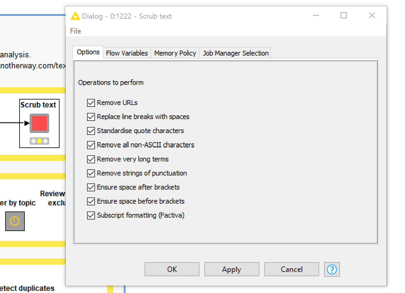
As is explained in more detail below, the TextKleaner facilitates four types of task to prepare your text data for analysis. The first is the cleaning or scrubbing of the text, which involves the replacement or removal of various characters in order to make the text more machine-readable. The second is the filtering of irrelevant documents. The third is the identification of duplicated documents and the removal of duplicated or ‘boilerplate’ text within documents. The fourth step includes both the enrichment of your texts through the tagging of named entities and ngrams, and the ‘optimisation’ of your texts via the removal of rare and uninformative words and the standardisation of plurals and other word variants. Other common preprocessing tasks, such as removing punctuation and standardising case, are performed along the way.

The TextKleaner can be applied to any genre of text data, though it’s worth mentioning that I have road-tested it mainly on news articles and submissions to public policy processes. The only firm requirement of your data is that it already exists in a tabulated format (such as CSV) and includes a document column formatted as a plain text string. Also keep in mind that this workflow is designed for collections of at least hundreds, and preferably thousands, of documents. Put simply, many of the techniques that the workflow employs rely on large numbers to work well. And let’s face it: if your collection doesn’t contain hundreds of documents, you probably don’t need any computational assistance to analyse it. ¹

When time allows, I hope to pull together some workflows that assist with the actual analysis of the textual data that you might prepare with the TextKleaner (thus far, the TopicKR is the only such example). But for the moment, this workflow is really for people who have their own means for performing such analyses — or for those who have commenced their own journey towards attaining those means.

The following sections explain at a high level how to use the TextKleaner. You will find further information about each component conveniently accessible within the workflow itself.

Installing the TextKleaner

To use the TextKleaner, you first need to download and install Knime. Then you can obtain the workflow by opening its page on the KNIME Hub and simply dragging the relevant icon into the Knime interface. As for exactly where you should drag it to, allow me to make the following recommendation.

Like my other workflows, the TextKleaner assumes that it will be just one of several workflows used to complete a project. For this reason, you should create a Workflow Group (in reality just an ordinary folder) for your project within your Knime workspace. Do this by right-clicking the LOCAL (Local Workspace) item in the KNIME Explorer and entering an appropriate name for your project. Then, drag the TextKleaner from the KNIME Hub into the workflow group that you have just created. If you import or create any other workflows to complete this project, be sure to place them in the same workflow group.

The advantage of grouping together project-related workflows in this manner is that they can more easily share project-specific data, including the data that each workflow produces. As with my other workflows, the TextKleaner will create a folder named Data within the project workflow group, and will save its output and throughput data there.

When you first install the TextKleaner, Knime might tell you that additional components need to be installed for it to work. This shouldn’t present any hurdles — just follow the prompts and you should be good to go. If the process has been successful, you should see something like this:

Loading your data

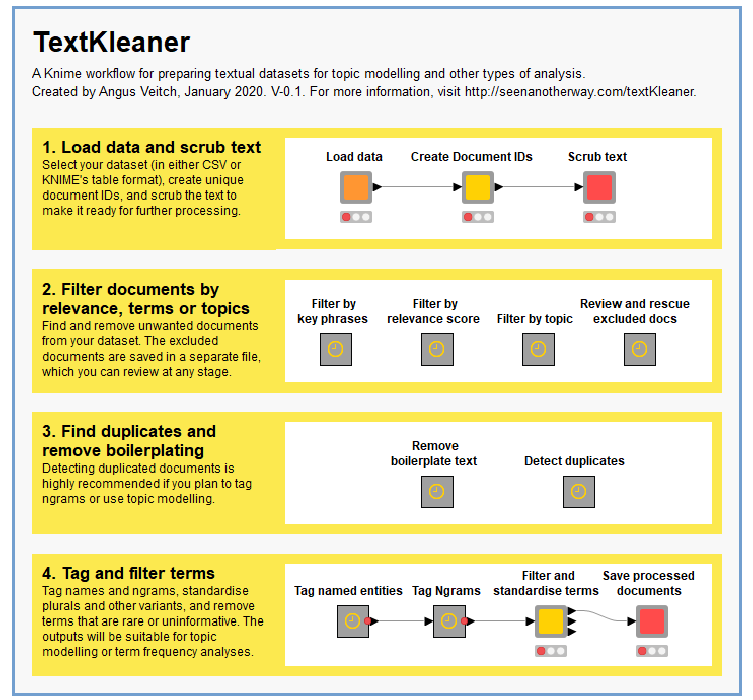
The TextKleaner assumes that you’ve already obtained your data and have wrangled it into either a CSV file or, preferably, Knime’s own .table format. To load your data into the workflow, double-click on the Load data node and use the config box to browse to your file. At this point, you will need to close the configuration box and attempt to execute the node. This will prompt the node to examine the input data, allowing you to configure the remaining settings. The most important of these settings is the Text column, as this tells the workflow which column of your input data contains the document texts, which must be formatted as plain text strings. Optionally, you can also specify columns containing the document titles and unique document identifiers. Finally, you specify which additional columns (if there are any in your data) you want to retain.

If your input file is a CSV, I can’t guarantee that this step will go smoothly. CSV files containing long text documents are notoriously unstable, and can require careful configuration (if not minor surgery) to load successfully. If the node fails to load your data, or if the loaded data (which you can see by right-clicking the node and viewing the output) appears to be corrupted, you will need to drill into the internals of the node (double-click it while holding down Ctrl) and play with the settings of the CSV Reader node until it parses your data successfully.

For the purposes of this demonstration, I will be loading and preparing a collection of news articles that I obtained from the Factiva database ² and converted into a tabular format with the help of my Facteaser workflow. The dataset contains just under 16,000 articles from Australian news outlets relating to the three-month lockdown that was enforced in the Australian city of Melbourne in response to a Covid-19 outbreak. (In case you’re wondering, the lockdown had a happy ending. After peaking at 687 daily cases on 4 August, Melbourne was Covid-free by 31 October, and, aside from one momentary hiccup, has remained that way until the time of writing.)

If you don’t have any text data of your own, you can still try out the TextKleaner by using the pre-loaded sample data, which should load by default if you run the Load data node. The sample dataset is a collection of 2,225 articles from BBC News, which I obtained from Kaggle.

Creating document IDs

The TextKleaner requires every document to be identified by a unique and unchanging string of characters. If your input data already includes an ID column for this purpose, feel free to specify it in the Load data node. If it doesn’t, or if you want to create new IDs, the Create Document IDs node will do this for you. This node will assign to each document a string of numbers preceded by a lowercase d — for example, d001, d002, and so on. The order of the numbers assigned will depend on the column that you specify in the node’s configuration. In this case, I chose to have the IDs follow the order of the Date column. The column that you choose here will make no different to your analysis; it’s merely a matter of convenience and aesthetics.

Scrubbing your text

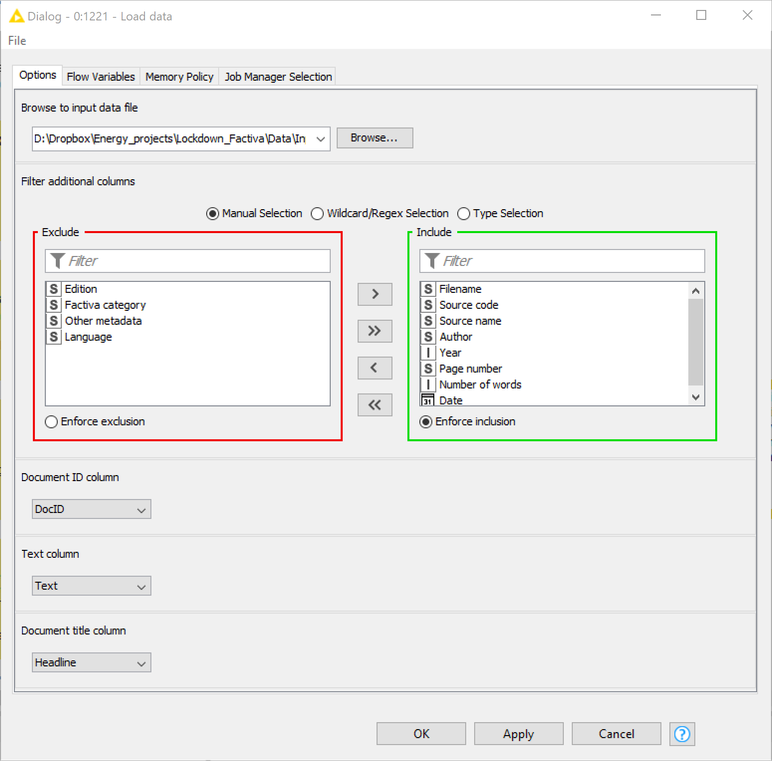
Depending on where your text has come from, you can almost guarantee that it will be riddled with things that you don’t want. Apostrophes that aren’t actually apostrophes; spaces that aren’t really spaces; floating punctuation or other symbols; weird characters that play no textual function at all; gibberish resulting from OCR or PDF artefacts — these are things that will only get in your way. Depending on your intentions, you might also want to be rid of things like URLs and line breaks. The Scrub text node addresses these issues, allowing you to choose from a list of replacements and removals that you might want to make. (Note that, as with some other nodes in this workflow, you may have to ‘nudge’ this node by executing it for a few seconds before the configuration options will become active.)

If there are additional scrubbing operations that you want to perform, and you are familiar with regex syntax, you can add as many operations as you want by opening the node (Ctrl+double-click) and editing the list in the Table Creator node that you will find inside.

Filtering out unwanted documents

Depending on how you acquired your data and what you plan to do with it, this step may be irrelevant to you. The reason why I have included not one but three different methods of excluding unwanted documents is that sometimes, acquiring a dataset is only the first step towards whittling it down to the dataset that you actually need to answer your research question.

This is frequently the case when you obtain your documents from a service that you query with keywords and other criteria. In this case, I obtained news articles from the Factiva service that mentioned the words lockdown,  covid* (or coronavirus) AND Melbourne. This query guaranteed that the articles will at least mention my topics of interest, but it didn’t guarantee that the articles will be about the Melbourne lockdown, and there’s a subtle but important difference between these two categories. Nor did my query restrict the type of articles that would be retrieved. It turns out that many of the articles in my collection were not news articles in the usual sense, but compendiums of posts from each day’s live blog coverage of coronavirus news — a format that seems to have become popular among online news services. In any case, I did not want to include the live coverage in my analysis, as it represented a completely different type of format from the traditional articles that made up the bulk of my collection.

The TextKleaner provides three methods for filtering out such unwanted documents: by key phrases, by relevance score, or by topic. I will describe each in turn.

Filtering documents by key phrases

The Filter by key phrases function (which you can access by opening up the relevant metanode) allows you to exclude documents that contain specified words or phrases. This method is useful if — and only if — the documents you want to exclude — and no others — can reliably be identified by their use of a specific word or phrase. In my case, I was able to remove nearly 4,000  live blog articles because they all started with introductions along the lines of “Welcome to live coverage of the continuing coronavirus crisis”. At the same time, I removed articles with the phrase “Industry snaphsot” in the title, since these were invariably of the type that I did not want to analyse.

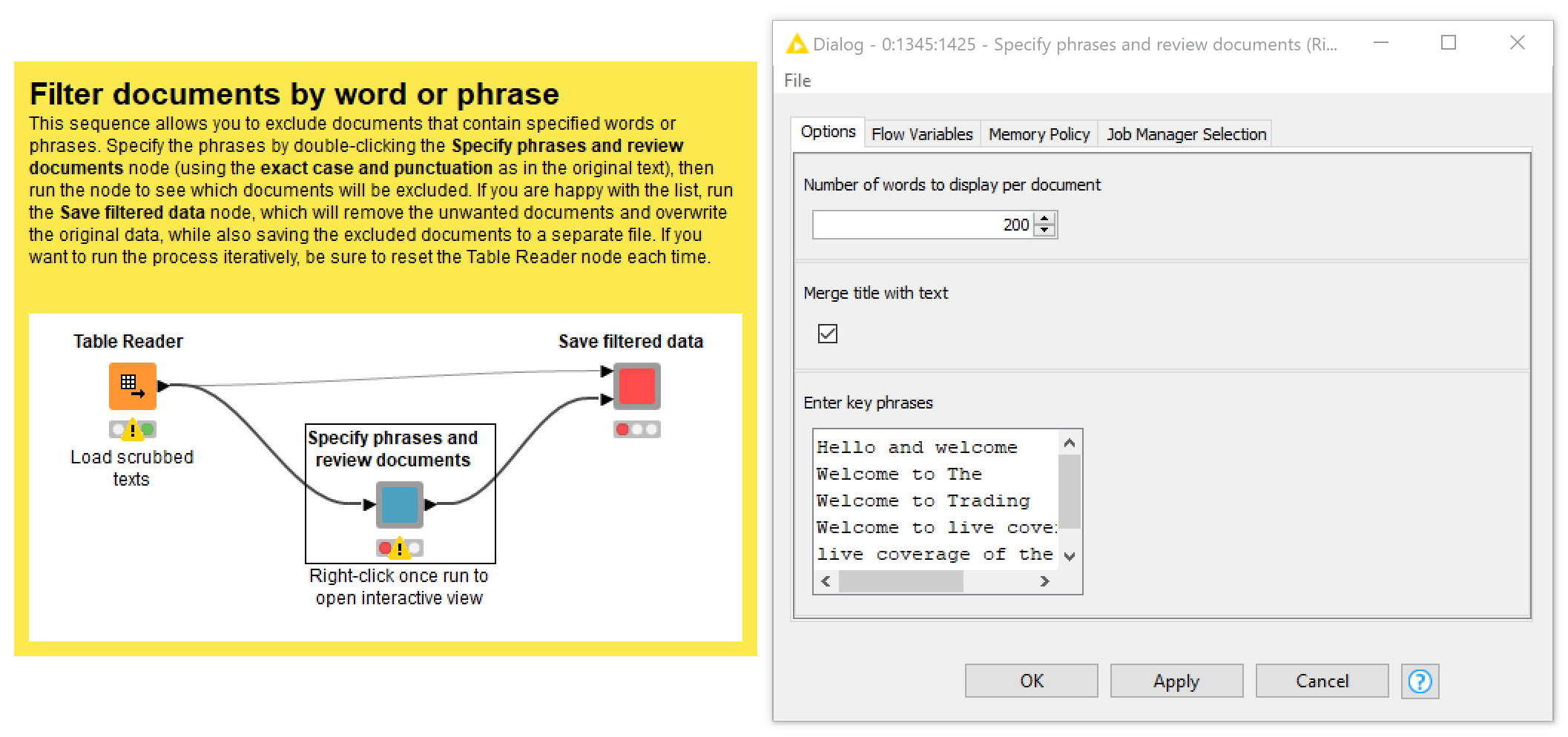
As per Figure 4, enter the incriminating phrases into the config of the Specify phrases and review documents node (note that the words or phrases that you enter here must be capitalised and punctuated exactly as they appear in the text), then run the node and view the relevant articles to make sure you want to remove them. If you’re happy with the results, run the Save filtered data node to save the results. As with most other operations in this workflow, this action will overwrite the file that was created by the text scrubbing step, or by any other steps that you might have performed first. This means that you can easily feed the filtered dataset back into this or any other operation by resetting the initiating Table Reader node. If you accidentally go too far and need to restore some excluded documents, you can do this in a separate part of the workflow, as is discussed a little later on.

Filtering documents by relevance score

In contrast with the key phrases method, the Filter by relevance score function enables you to exclude documents that don’t include specified words — or more specifically, that don’t mention them early or often enough. You could call this a measure of ‘aboutness’, because it separates documents that merely mention a given topic from those that are clearly about the topic.

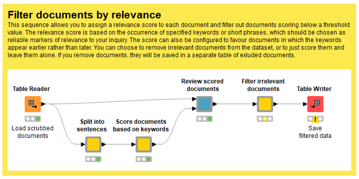
To use this method, you need to be able to specify a list of keywords that, collectively, are highly reliable indicators of your topics of interest. Unless at least one of these words appears fairly early on in a given document (or possibly many times later on), that document will be assigned a low relevance score. Once you have specified these words in the config of the Score documents based on keywords node, run the Review scored documents node and use its interactive view to see how how the documents have been scored. At this point, you can choose to remove all documents that score below a threshold value, or to just append the scores to the table in case you want to use them later.

Filtering documents by topic

Sometimes, especially if you’ve obtained your data through a keyword search, you end up with documents about topics that are completely unrelated to your interests. The Filter by topic function provides a way to find and remove these documents. It does so by first generating a topic model of your dataset. This means that it finds groups of words that are frequently used together in your texts — these are the ‘topics’ — and estimates the extent to which each topic is present in each document. This makes it easy to identify and remove documents that consist mostly of irrelevant topics.

Topic modelling can be a time-consuming process, which is why I suggest removing unwanted documents by any other means possible first. Something else that you might want to do first is to identify duplicate documents in your data, using the function described in the relevant section below. If the duplication results are available to the Filter by topic function, the function will use this information to exclude duplicates from the topic modelling process, thereby executing faster and producing more meaningful topics. For a similar reason, you may also want to run the boilerplate removal step before this one. Because topic models work by finding words that occur together, they will generally produce better results if you remove as much uninformative co-occurrence (such as duplicated documents or boilerplate text) as possible.

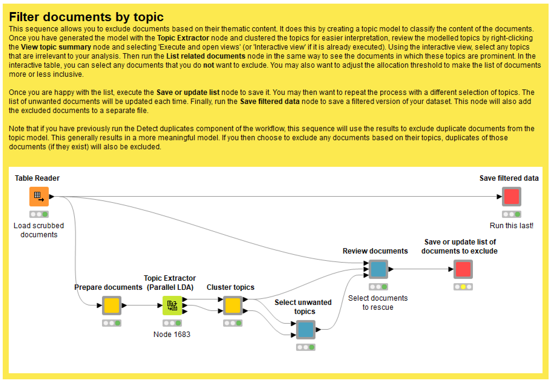
As you can see in Figure 6, there are several steps involved in this task.

The Prepare documents node performs various preprocessing steps such as removing punctuation, standardising case, and filtering out rare or uninformative words. You can tweak a few parameters here, such as how rare or common a term has to be to warrant exclusion. And in case you’re worried, keep in mind that this step will not alter your original documents; this preprocessing is purely for the sake of building the topic model.

The Topic Extractor node then uses LDA, a popular topic modelling algorithm, to create a topic model from your documents. The only parameter that you should worry about here is the number of topics. More topics will increase the processing time and increase the interpretive load, but will also allow you to be more specific about what you filter out.

The Cluster topics node then rearranges the topics into thematic groups, the number of which you can specify in the configuration. (If you want to, you can also specify whether topics are grouped together based on their terms or their document allocations, but honestly I wouldn’t worry too much about these settings.) This just makes the topic model easier to interpret and review, which you’ll do in the next node.

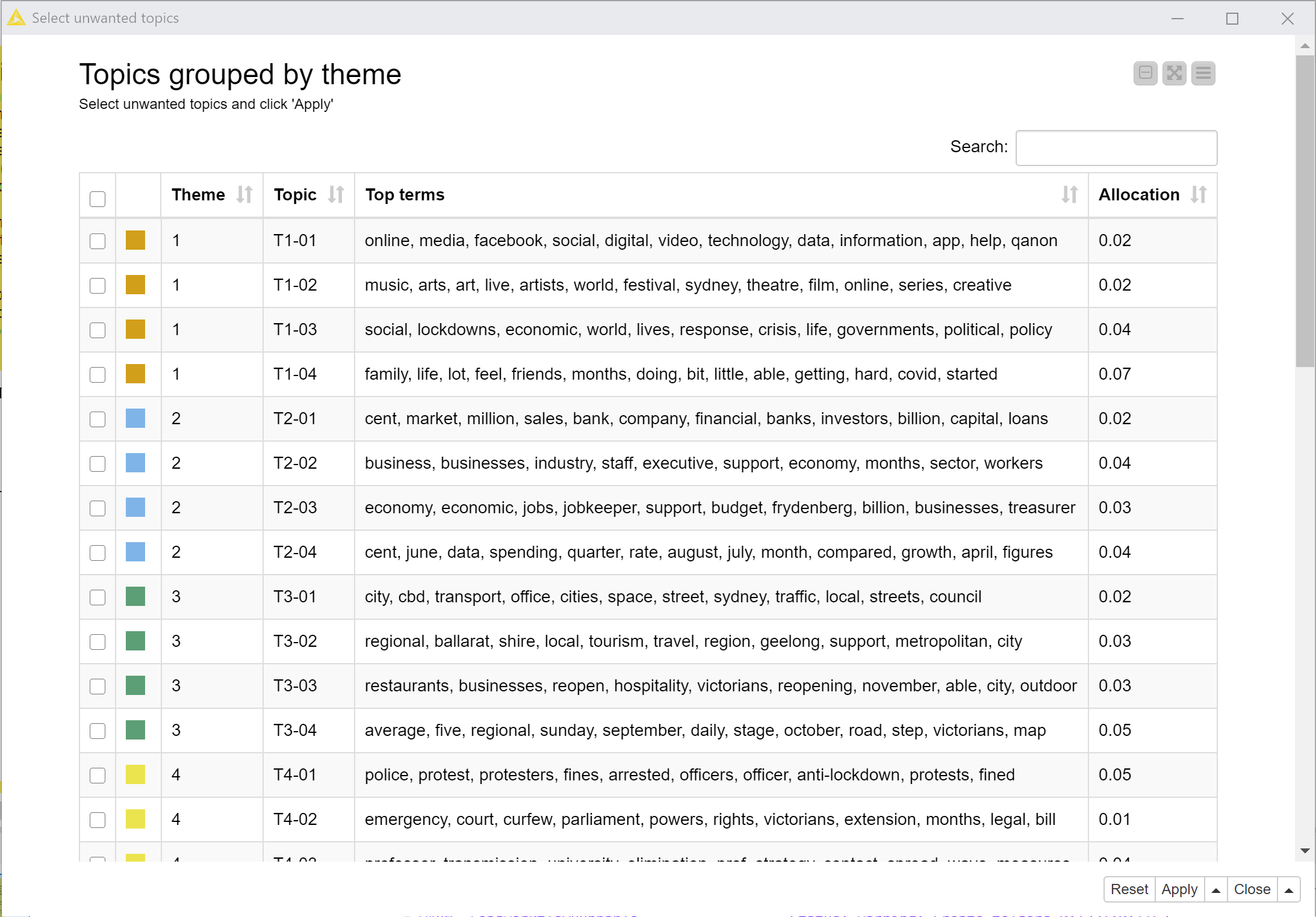
Executing and opening the interactive view of the Select unwanted topics node will produce a table summarising all of the topics discovered in your data. Figure 7 provides an example. In this case, there weren’t many irrelevant topics left, but I did notice one topic that appeared to be about the media (its top terms included abc, media, news, pell, journalists, readers, and radio) rather than anything directly related to the lockdown. So I selected this topic, clicked ‘Apply’, and moved onto the next node.

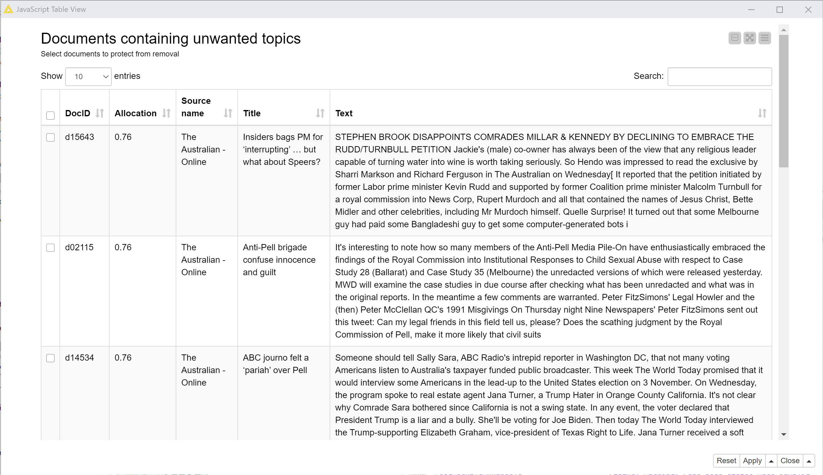
The Review documents node provides an interactive table showing excerpts of all documents in which the selected topics are prominent (where prominence is defined by a threshold allocation value). The example in Figure 8 shows that in my case, many of the articles dominated by the selected topic were pieces from The Australian and the Herald Sun (the national and Melbourne outlets of News Corp) discussing journalists and media outlets, generally to attack other outlets’ journalists or to congratulate their own. Many, but not all, were indeed only tangentially related to the lockdown. To retain any relevant documents shown in this view, just select them and click ‘Apply’ before executing the next node.

The Save or update list of documents to exclude node does exactly what it says. When you run this node, it creates or extends a list of documents that should be excluded based on their topical content. Once you have executed it, you can go back to the Select unwanted topics node and select a new batch of topics to review. Each time you repeat the process, the results will be added to the exclusion list. If you want to wipe the slate clean and start the process again, select the ‘Start new list’ option in the Save or update list node — but remember to unselect it afterwards if you want to build the list in multiple steps.

Once you have identified all the documents you want to remove, run the Save filtered data node to remove these documents from the dataset.

Reviewing and rescuing excluded documents

When removing documents from your collection, it’s easy to go a bit too far and remove things that, on second thoughts, you want to keep. The Review and rescue excluded docs function provides a way to retrace your steps and restore any documents that you might have removed by mistake. Its interface works in much the same way as the filtering functions. The Review excluded documents node will generate an interactive list of documents that have been excluded, showing an excerpt of each document’s text and specifying the filtering process in which it was removed. Select any documents that you want to restore, click ‘Apply’, then run the following node to restore them to your active dataset. Just be mindful that if you have run the boilerplate removal or duplicate detection functions since removing a document, this document will not have been seen by those functions if you restore it.

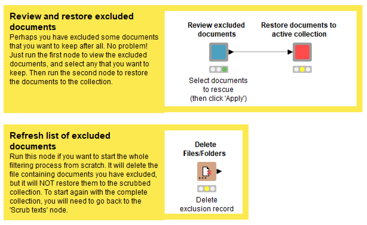
If you want to start the whole filtering process again, make sure you run the Delete Files/Folders node, as this will delete the list of excluded documents. If you don’t do this, your record of excluded documents will retain the results from the previous filtering process.

Removing boilerplate text

This is another function that might be totally irrelevant to your data. But if you are dealing with texts such as news articles or academic papers, you are likely to find that many of your documents begin with chunks of text that is repeated verbatim in other documents. This is an example of what is often called boilerplating, or boilerplate text. As its name suggests, the Remove boilerplate text function attempts to detect and remove such text from your documents. For the moment, it only removes such text if it occurs at the start of your documents, rather than the end. I hope to update the TextKleaner soon to include the latter capability.

The method that the TextKleaner uses to do this is pretty experimental, so always be sure to review the results before saving them. It works by finding short stubs of text that are repeated across several documents (the length of these stubs and the number of documents are configurable), and then scanning ahead to determine where the boilerplating ends and the unique content begins.

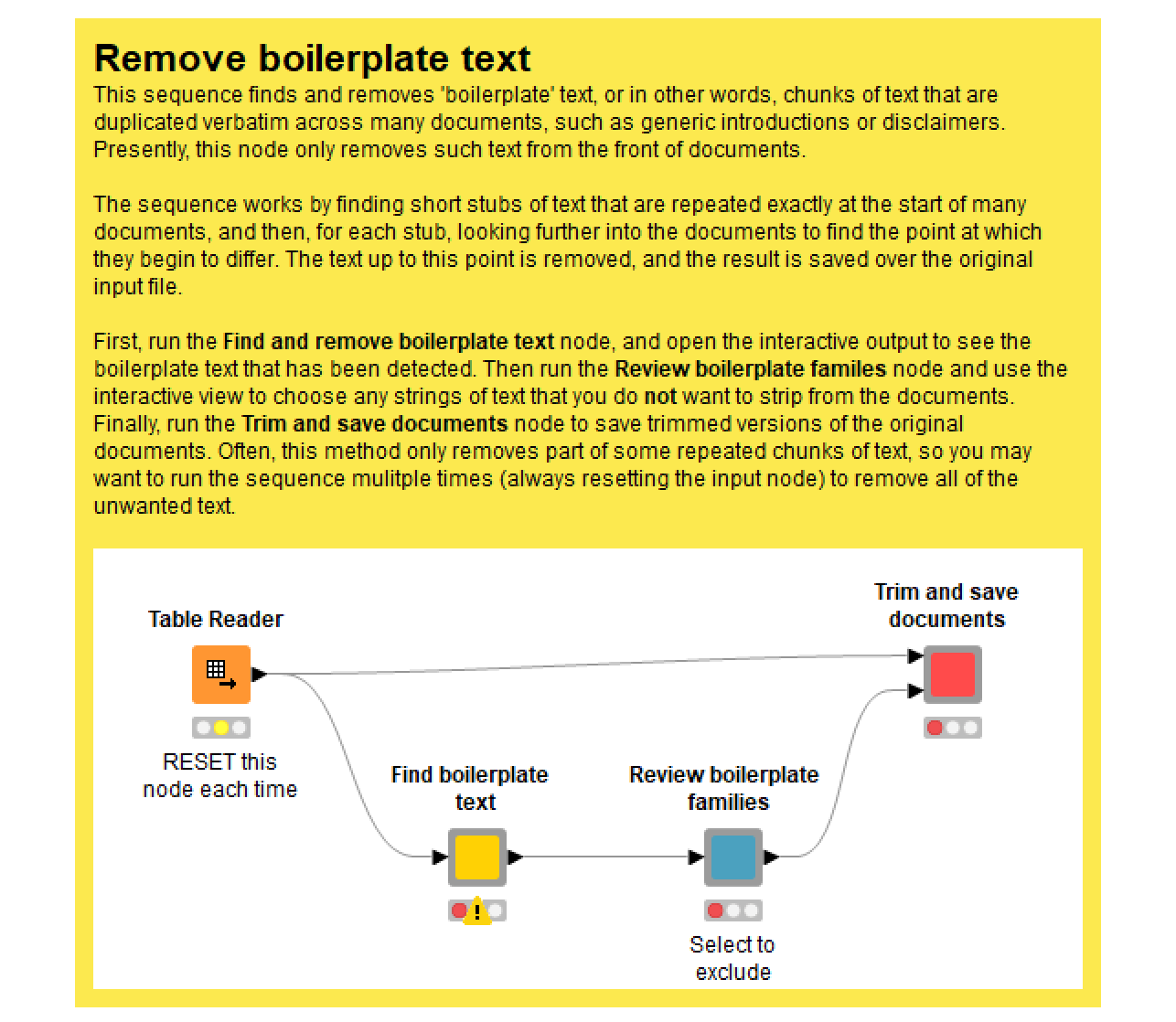
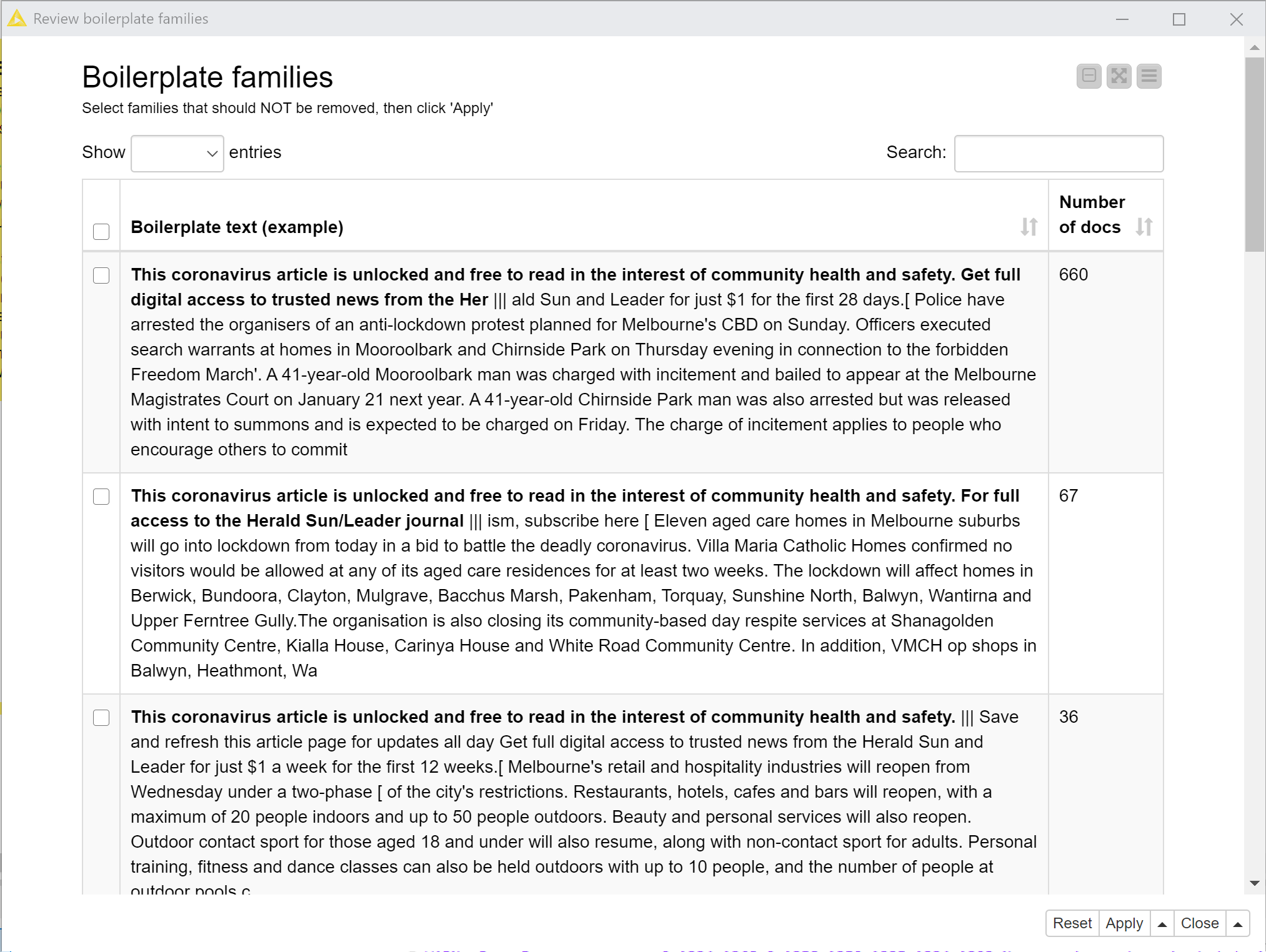
When you execute and open the interactive view of the Review boilerplate families node, you will see a list of text excerpts, each of which illustrates a unique piece of boilerplating that is repeated across many documents. As per the example in Figure 11 (in which the boilerplate text is in bold), these boilerplate ‘families’ are often variants of one another. Sometimes, however, they are not really boilerplating at all, but are legitimate content that just happens to be recycled. To ignore these families, select their table rows and click ‘Apply’.

Running the Trim and save documents node will then remove the bold segments of text (unless they were selected in the interactive view) from the documents in which they appear, and overwrite the input dataset.

There is a good chance that you are not finished yet. If you look closely at Figure 11, you’ll notice that the bold text doesn’t cover all of the text that should be removed. This is because the boilerplate identification method takes a conservative approach to avoid removing legitimate content. To clean up the remaining boilerplate text, just run the process again (perhaps a few times), taking care to reset the Table Reader node each time.

As noted earlier in relation to the Filter documents by topic function, it’s a good idea to remove boilerplating before you use that function, as it will generally result in a better topic model.

Detecting duplicated documents

Some types of text data, such as news or Twitter posts, tend to be littered with documents that are very similar to one another, if not completely identical. Such duplication might be of interest to your analysis, or it might be an annoyance. In either case, keeping track of duplication at the document level is a useful thing. Tracking duplication is also useful if you plan to analyse term frequencies or co-occurrences, or to use topic modelling, as extensive duplication can cause these methods to produce confusing or misleading results.

The TextKleaner includes a function that identifies families of duplicated or very similar documents. It doesn’t remove the duplicates, but instead saves a separate file specifying whether each document is unique, a master with copies, or a copy. If a document is a copy, the output specifies the ID of its ‘master’ document. In each family of duplicates, the master document is the one with the largest amount of shared content.

At a theoretical level, detecting duplicate documents is not a difficult computational problem to solve. What is difficult is doing it efficiently. There are lots of academic and technical papers about the topic (and I’ll admit, many of them are above me), but as far as I can tell, there are not many tools available for performing the task — and certainly nothing ready-made for Knime.

As it happens, one of my very first posts on this blog was an experiment in duplicate detection that matched documents using nothing more than a handful of function words — words like it, the, and, be, or of, which are typically removed from semantic analyses of texts. For the TextKleaner, I have used a method that is more computationally expensive but also much more accurate. In essence, it works by removing all but a few hundred unique terms from the documents, then creating ngrams (sequences of words) out of what remains, and comparing documents based on the ngrams that they contain. I have no doubt that there are smarter duplication detection methods methods out there, but this approach seems to work quite well, and is not so slow as to be impractical. It took my laptop about 12 minutes to identify the approximately 7,000 non-unique documents in my filtered dataset of 11,485 documents. If your collection contains less duplication than this (or if your documents are shorter), the process should be much faster, as the method only compares documents that contain a certain amount of shared material.

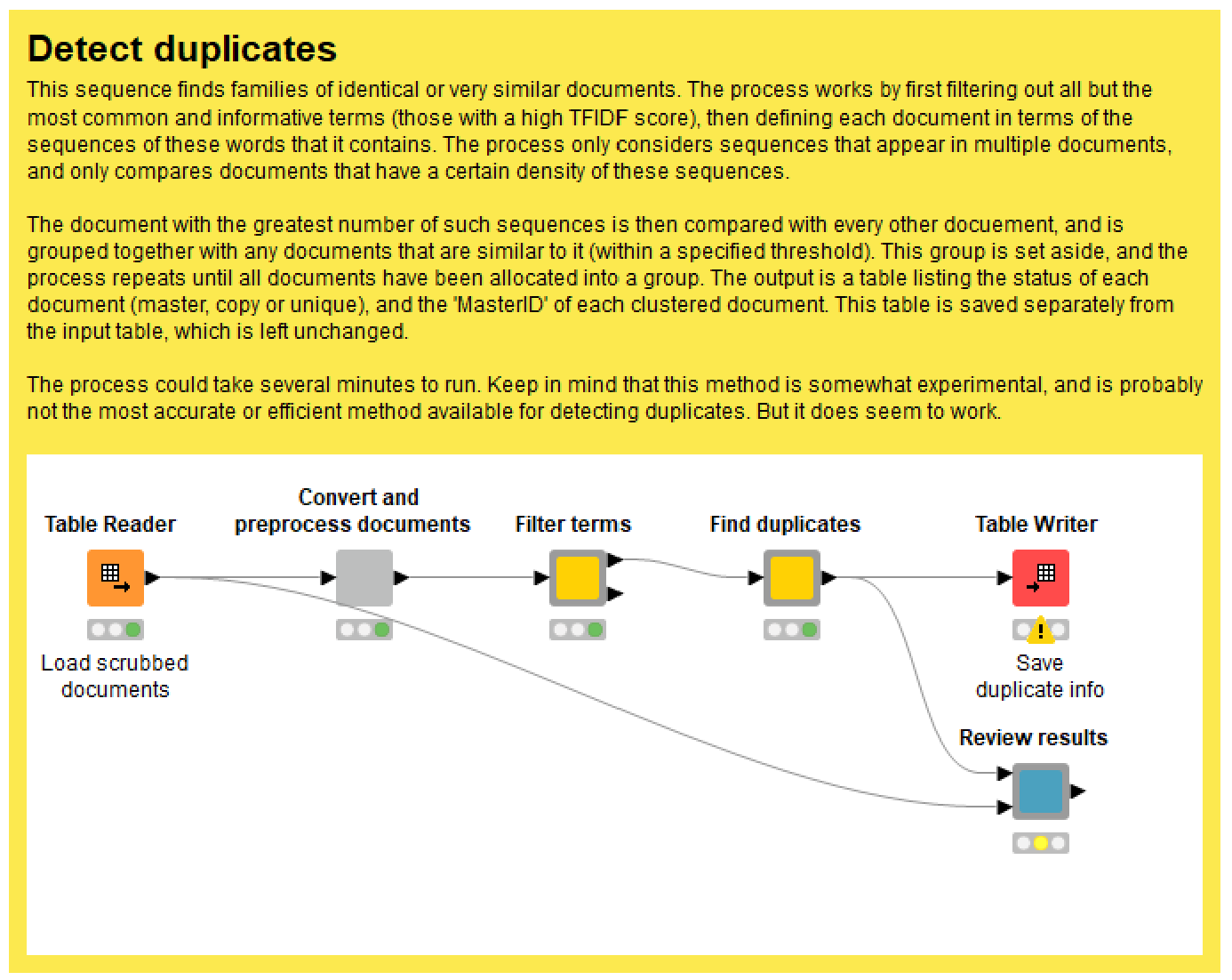
The duplicate detection function provides a handful of configuration options. First, you can choose the number of unique terms to retain in the documents. The goal is to make this number as small as possible while ensuring that all documents still contain enough terms to enable similarity measurements. This information can be found in the second output of the Filter terms node. The settings in the Find duplicates node let you change the length of ngrams used to compare documents, the minimum percentage of shared ngrams that a document must contain to be included in the analysis, and the level of similarity that defines a duplicate.

When the detection process is complete, you can use the Review results node to check that the results make sense. Finally, run the Table Writer node to save the duplication information as a separate file, which will be accessed by other parts of the workflow as required. The TextKleaner keeps these results in a separate file so that you don’t have to run the duplicate detection process again, even if you decide to re-start the rest of the filtering and cleaning process from scratch.

If you do end up removing documents after detecting duplicates, you may want to run the duplicate detection process again to make sure that the saved duplicate information pertains only to the documents in your collection. This should not be essential, but I suggest doing it just to be sure.

Tagging and filtering terms

The steps described above are mostly aimed at cleansing your data of unwanted information, whether by removing or replacing unhelpful characters, filtering out unwanted documents, trimming boilerplate text, or keeping track of duplication. The remaining steps are a little different. They include the enrichment of your data through the tagging of names and ngrams, and its optimisation through the removal or standardisation of specific terms that are not needed or wanted in your analysis.

While there was some flexibility in the order in which the preceding steps were performed, these final steps must be performed in the prescribed order, and, unless you really know what you are doing, should be done only after you have finished with all of the preceding steps. You can, however, skip any of these final steps by following the instructions in the workflow.

When these last steps are completed, the TextKleaner will create a new output file that encodes your processed documents as tokenised sequences of whole terms, rather than as strings of characters. All terms will be converted to lowercase unless they are tagged as names, and all punctuation will be removed. The purpose of this rather savage treatment is to prepare your documents for topic modelling, term frequency analyses or other analytical techniques that rely on a bag-of-words model of text. At present, the TextKleaner is not set up to output tokenised documents that include punctuation or sentence boundaries, although you could modify it to do this without much difficulty. If there is interest in this functionality (or if I happen to need it!), I may add it in a future revision of the workflow.

One final thing to consider is that the output saved by this part of the workflow uses Knime’s native tokenised document format. If you want to use other software to analyse your preprocessed documents, you will need to export the tokenised documents to a more universal format. The easiest way to do this is to use the Document Data Extractor node to extract the document text as a plain text string. However, unless you have used a carefully chosen separator (like a 7) to replace spaces in your tagged names and ngrams, these entities will fragment into their constituent parts in converted text string. Even if you do keep them joined together, you will still lose the tags that designate their entity type. If you want to retain this information as well, you could try converting your documents into a table so that every word has its own row with a column designating its entity type. If you don’t care about word order, the Bag of Words Creator node (perhaps in combination with the TF node) will do this for you. If the word order AND entity tags are important, then as far as I know, you’re stuck until Knime adds more functionality to the text processing nodes.

Tagging named entities

Distinguishing names from ordinary words can be useful for various reasons. If you want to analyse the references to people, places or organisations in your data, these names need to be tagged so that each name can be counted as a single term. They also need to be classified, not only so that names can be separated from words, but also so that the names of places, people and organisations can be distinguished from one another. On the other hand, if you don’t want to analyse names, then tagging them will enable you to exclude them from your data, leaving just the ordinary words.

Knime’s collection of text processing nodes includes two named entity taggers, one from the Stanford Natural Language Processing (NLP) Group, and the other from the OpenNLP toolkit. Straight out of the box, both taggers do a pretty good job of detecting names and guessing whether each is a person, place or organisation. (I generally use the StanfordNLP tagger, if only because it can tag all types of entities in a single pass.) However, the results are usually far from perfect. A close inspection usually reveals many instances where names have been misclassified (a person, for instance, is tagged as a place) or not tagged at all.

For this reason, I like to use the results from the named entity tagger as a starting point from which to create a tagging dictionary, which is simply a list of names and associated entity types. The tagging dictionary can be used to find every instance of every name, thereby catching all the instances that the named entity tagger misses. The downside of this approach that it only allows each name to assume a single entity type, so that if your data includes references to Victoria the place as well as a person named Victoria (for example), you won’t be able to separate them unless the full name of the person is used. Usually, however, I find that forcing a single entity type per name corrects many more errors than it causes.

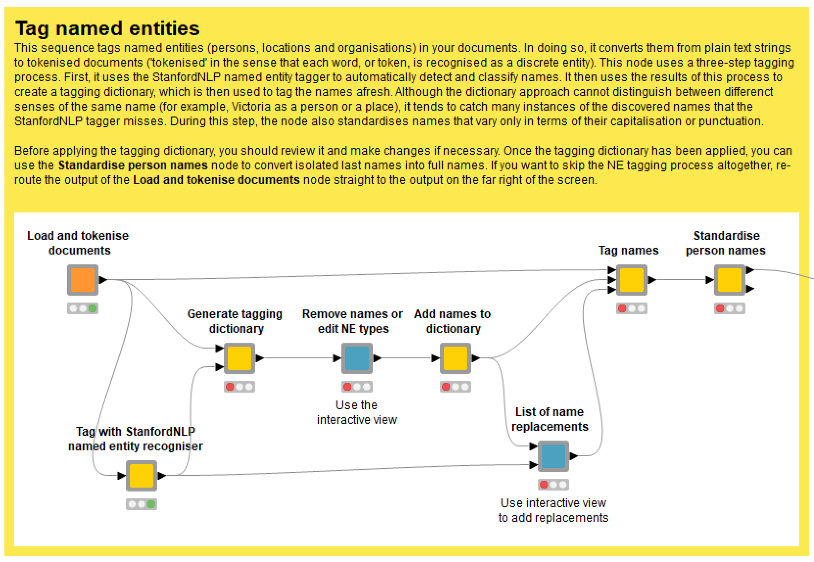
As per Figure 13, the tagging dictionary is assembled in several steps. First, the Generate tagging dictionary node uses the output of the StanfordNLP NE Tagger to create a draft list of names with assigned entity types. In making this list, the node does its best to standardise variants of the same name, recognising, for example, that Daniel Andrews, Daniel ANDREWS and DANIEL Andrews are all likely to be the same person. The most common variant of each name is assumed to be the preferred version. Similarly, the entity type that is most commonly applied to a given name (including variants) is selected as the entity type for all instances of that name. In this step, you can configure the maximum number of parts that a name can have (since the StanfordNLP tagger sometimes erroneously tags very long chains of words as names), and a threshold ‘capitalisation ratio’ value that will prevent words that are rarely capitalised from being tagged as names, even in their capitalised form (common examples are Earth and directions such as North East).

By default, these calculations are based on tallies of the total number of occurrences of every term. However, since these term frequency calculations can be painfully slow to run, the node also gives you the option of using document frequencies (the number of documents in which each term occurs) instead. While much faster, document frequencies may produce poorer results, so I recommend using them only if term frequencies take too long to compute.

Once the draft dictionary has been generated (and please be patient, as this can take some time), use the subsequent nodes to add and remove names from the dictionary, or to edit the assigned entity types.

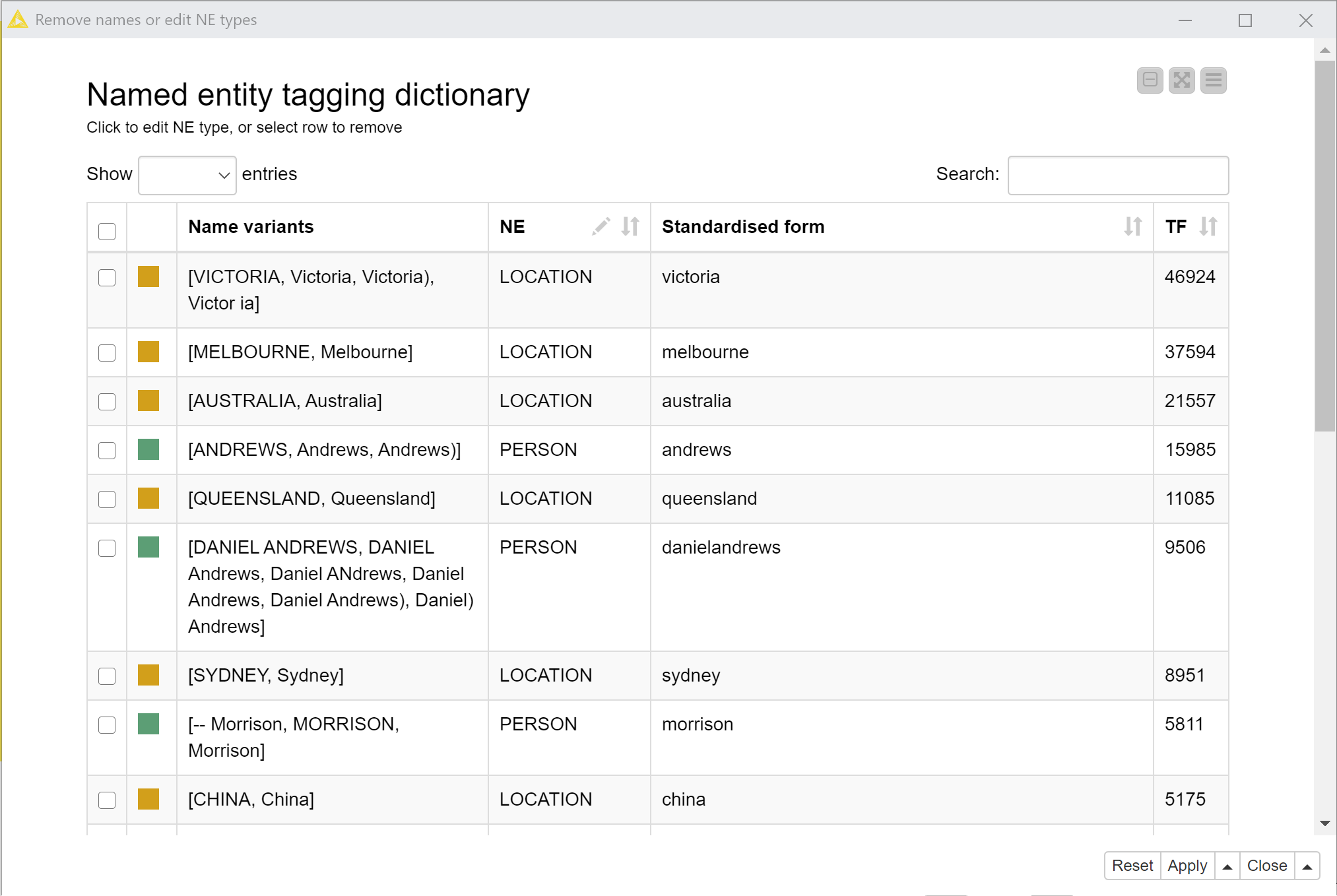
Figure 14. An excerpt of the automatically generated tagging dictionary. In this view, you can select names to remove, or edit the entity types.The List of name replacements node shows which name variants will be replaced with which, and also allows you to add replacements of your own. In this case, for example, I added Daniel Andrews as a replacement for Dan Andrews.

Once the tagging dictionary and name replacements are finalised, run the Tag names node to tag the names in your documents. By default, the spaces in multi-part names will be replaced with underscores (so Daniel Andrews becomes Dan_Andrews). This is largely an aesthetic decision, so, for example, multi-part names can be clearly distinguished in lists of top terms. However, it is also an insurance policy against such names being fragmented in any future processing steps. Note that in the latter case, I have found that some text processing operations in Knime will still separate words that are joined by an underscore. If this is an issue, you may want to use a non-punctuation character (I usually use a ‘7’) as a separator, which you can do by changing the configuration of the Tag names node. If you prefer, you can specify an ordinary space instead.

Once the names in the dictionary have been tagged, the TextKleaner offers one final (and optional) layer of standardisation. If activated, the Standardise person names node will make an effort to replace isolated last names, including those preceded by a title such as Mr or Dr, with the full version of of the names. For example, in my data, it will convert some — but not necessarily all — instances of Andrews or Mr Andrews to Daniel Andrews.

To decide which names to convert, and what names to convert them to, this node pays attention to the thematic context of the names. It does this by building a topic model consisting of names and a limited number of ordinary words. The modelled topics (which are essentially ranked lists of words and names) reveal which names (complete or partial) tend to occur in association with specific topics. Meanwhile, the topic model estimates the presence of each topic in each document. This information is combined to guess which full name should be substituted for each partial name. In my dataset, Mr Andrews would almost certainly refer to Daniel Andrews in any document that discusses the Victorian Government (of which Daniel Andrews is the leader). But if my dataset had included a batch of documents about The Sound of Music, there is a good chance that the topic model would have tagged these documents with a separate, music-themed topic containing the name Julie Andrews, and that this name would replace any instances of Andrews in those documents.

Like many methods in the TextKleaner, this name standardisation technique is somewhat experimental, but it does seem to work pretty well.

Tagging ngrams

Names are not the only sequences of words that we may wish to count as single units. In any textual dataset, there are likely to be sequences of two or three (or perhaps more) words that appear over and again, and that mean something distinct from their component parts. If we were to analyse a collection of articles about text analysis, for instance, we would probably want to count the phrase text analysis as a single term, rather than counting the words text and analysis separately.

Terms consisting of multiple words are often called ngrams (where ‘n’ is a placeholder for the number of words in the sequence), and, if selected carefully, can greatly enrich a bag-of-words style textual analysis. Deciding which ngrams to tag, however, is no simple matter. Working your way down from the most frequently occurring ngrams is a reasonable approach, but when you look closely, you start to discover that the most frequent ngrams are not always the most interesting ones, and that some of the rarer ngrams can be highly informative.

The Tag Ngrams function of the TextKleaner uses a combination of frequency and co-occurrence statistics to generate an automatic (but editable) list of ngrams to tag in your documents. In addition to the overall frequency of each ngram, it considers the normalised pointwise mutual information (NPMI) of its terms. Roughly speaking, the NPMI of an ngram is a measure of how surprised we should be when we see it, given how often each of its constituent words occur (and assuming we know nothing about the subject matter). A high NPMI score can be taken as evidence that the words in an ngram are being used together very deliberately and systematically.

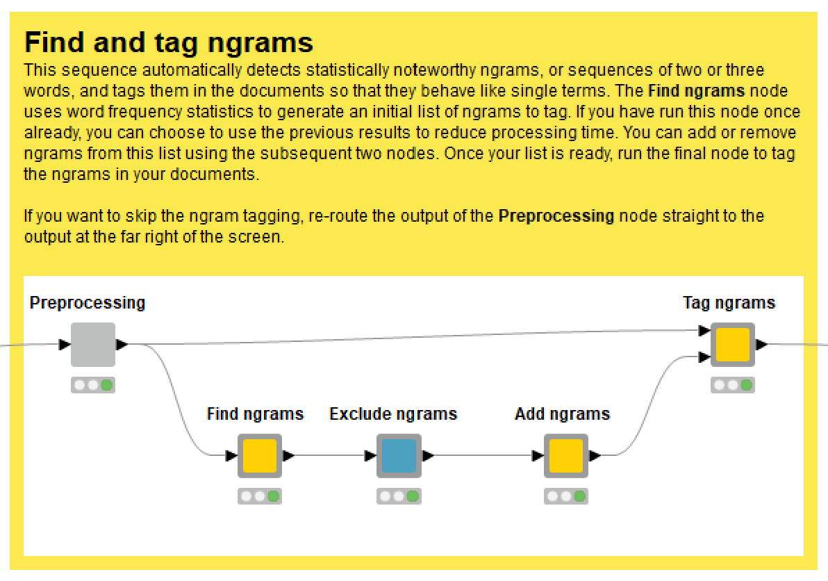
To prepare your documents for this process, the Preprocessing node erases all punctuation and converts all words not tagged as names to lowercase. Even if you opt not to tag ngrams in your data, you must still run this node. Otherwise, the subsequent term filtering and standardisation process will not work.

The sensitivity of the automatic ngram detection process can be controlled via the settings of the Find ngrams node. If you have already run this process on your dataset once before, this node also gives you the option of using the previously generated list of candidate ngrams to save you generating the term frequency statistics again.

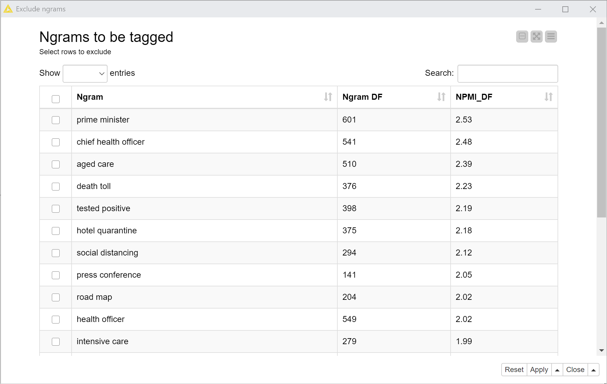
The Exclude ngrams node enables you to review the discovered ngrams and to remove any that you do not want to tag, while the subsequent node allows you to add ngrams that are not on the automatic list. Finally, the Tag ngrams node tags all instances of the listed ngrams, replacing the spaces between words with underscores or some other specified separator.

Filtering and standardising terms

If you’ve made it this far, you’re nearly finished. With all the relevant names and ngrams tagged, it’s time to optimise your data to ensure that it contains only the information that you care about. This means, firstly, removing terms that are either so common that they are unhelpful, or so rare that they won’t have any impact on your analysis. The thresholds for these actions can be set in the configuration of the Filter and standardise terms node. To determine intelligent values for these thresholds, I suggest running the node with the default values first, then reviewing the results in the second two output ports, and if necessary, running the node again with revised thresholds.

This node will also remove stopwords such as to, be, or the, which have no place in most bag-of-words style analyses. In addition, you can specify your own list of words to be removed.

As well as removing unwanted terms, this node standardises some word variants such as plurals or past tense, so that, for example, vaccines might become vaccine, or protested might become protest. I say ‘might’ because the standardisation method used in this node will only replace variants if they are sufficiently rare compared with the root form, and if they occur in association with the same topic (yes, this node also builds a topic model!) as the root form. What this amounts to is a very gentle form of lemmatisation, which in turn is a gentle form of stemming, which in my opinion is a technique that you would only ever apply if your outputs were never meant to reach human eyes. Because of the time required to apply this standardisation technique, this node gives you the option to re-use the generated replacements list in subsequent executions. (To review the replacements list, you’ll have to dig down into the node. In a future revision, I’ll try to make this list more accessible.)

Conclusion

There’s no getting around the first law of text analytics. Analysing text with computers will always be really hard. I hope, however, that the TextKleaner makes some aspects a little easier. As with many forms of data analysis, the preparation of text data really is a large part of the battle, and the TextKleaner provides solutions to various text preparation problems that have drained a lot of my time and energy in the past. These solutions are by no means definitive: each represents just one of many possible ways in which the problems could be tackled, and all of them are skewed towards the types of analyses that I have spent my time doing. Hopefully though, these methods and the way in which they are packaged are sufficiently generic that they will be of use to other practitioners.

In sharing this workflow, I also hope to have advanced the case for using Knime as a platform for textual analysis (and indeed for data analysis more generally). At the end of the day, Knime will not be the most flexible or powerful platform for this purpose, as it is limited to specifically packaged versions of software libraries that are native to other platforms, such as R or Python. The use of a graphical interface instead of a coding language also limits what can be done in Knime (although to nowhere near the extent that you might assume). But despite such limitations, Knime has something that the other platforms lack — namely, accessibility. Text analytics is hard enough as it is; there is no need for it to be made harder by having to learn how to code, which is a prospect that, rightly or wrongly, is simply too confronting for many people with no training in computer science.

At this stage, I don’t know what the future of the TextKleaner will be. I hope to periodically update and improve it, but the extent to which that happens will depend on how many other people use it and how much time I have to spare. If you do use the TextKleaner, please do credit me in whatever way is appropriate, such as by citing my name (Angus Veitch), this page, and/or the workflow’s home on the KNIME Hub. And if you have any questions or feedback, feel free to drop me a line.