In the posts I’ve written to date, I’ve learned some interesting things about my corpus of 40,000 news articles. I’ve seen how the articles are distributed over time and space. I’ve seen the locations they talk about, and how this shifts over time. And I’ve created a thematic index to see what it’s all about. But I’ve barely said anything about the articles themselves. I’ve written nothing, for example, about how they vary in their format, style, and purpose.
To some extent, such concerns are of secondary importance to me, since they are not very accessible to the methods I am employing, and (not coincidentally) are not central to the questions I will be investigating, which relate more to the thematic and conceptual aspects of the text. But even if these things are not the objects of my analysis, they are still important because they define what my corpus actually is. To ignore these things would be like surveying a large sample of people without recording what population or cohort those people represent. As with a survey, the conclusions I draw from my textual analysis will have no real-world validity unless I know what kinds of things in the real world my data represent.
In this post, I’m going to start paying attention to such things. But I’m not about to provide a comprehensive survey of the types of articles in my corpus. Instead I will focus on just one categorical distinction — that between in-house content generated by journalists and staff writers, and contributed or curated content in the form of readers’ letters and comments. Months ago, when I first started looking at the articles in my corpus, I realised that many of the articles are not news stories at all, but are collections of letters, text messages or Facebook posts submitted by readers. I wondered if perhaps this reader-submitted content should be kept separate from the in-house content, since it represents a different ‘voice’ to that of the newspapers themselves. Or then again, maybe reader’s views can be considered just as much a part of a newspaper’s voice as the rest of the content, since ultimately it is all vetted and curated by the newspaper’s editors.
As usual, the relevance of this distinction will depend on what questions I want to ask, and what theoretical frameworks I employ to answer them. But there is also a practical consideration — namely, can I even separate these types of content without sacrificing too much of my time or sanity? 40,000 documents is a large haystack in which to search for needles. Although there is some metadata in my corpus inherited from the Factiva search (source publication, author, etc.), none of it is very useful for distinguishing letters from other articles. To identify the letters, then, I was going to have to use information within the text itself.
Using words to find letters
Helpfully, some newspapers began the relevant columns with headings like “YOUR LETTERS” OR “HAVE YOUR SAY”, or ended them with consistently worded instructions for readers wanting to submit their contributions. Using the text processing features in Knime, I scored every article by the presence of these markers, and this way identified around 800 letters. But not all letters included such helpful markers as these. I was going to have to get more creative if I was to use an automated method to find them.
For a human reader, distinguishing between letters and news stories is in most cases trivially easy. They often end with the sender’s name and place of residence — something I could no doubt train the computer to do, but I’m leaving that challenge for another day. Letters are also usually written in first person, and in language that is less formal and more emotive than news articles. This is something I felt I could probe with my existing skillset. I came up with a bunch of markers that I thought would be much more likely to appear in letters than in other kinds of content, and used Knime to count the frequency of these markers in every document in the corpus. These markers included pronouns like “I”, “we”, “our” and “you” which I felt were reasonable markers of informal language, as well as exclamation marks (!) and question marks (?). Using the frequencies of these markers, I then compared the 800 letters I had already identified against the remaining unclassified articles:
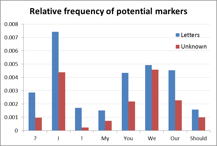
My hunch was correct: with the exception of “we”, these markers were on average much more prevalent in the letters than in the remainder of the corpus (most, but not all, of which was content other than letters). The exclamation mark appeared be an especially strong marker, appearing on average seven times more frequently in the letters than in the rest of the corpus.
Using a machine to make things more complicated
If I was to do all this again, I would have looked for a statistical or machine-learning approach to identify markers like these automatically. But there are only so many completely new things that I’m willing to experiment with at once. As it happened, I took the opportunity to dabble in machine learning in the next step of the process, which involved using these markers to find more letters.
Rather than simply sorting the corpus in order of the prominence of the markers and classifying new letters manually, I decided to see what I could do with Knime’s Support Vector Machine (SVM) functionality. An SVM is a supervised machine learning technique finds or ‘learns’ the distinguishing features of different classes of objects within a set of training data, and then uses this information to classify the objects in an unclassified dataset. I’ll happily admit that I am way out of my depth in using this technique, but I was convinced that in principle, it was suited to my task. I had a training set of documents that I knew to be letters (which I padded out with an equivalent number of non-letters), a large set of unclassified documents, and a set of parameters (the pronoun and punctuation markers) with which I could train the SVM. I figured that at the very least, the SVM would generate a tight pool of candidates for manual classification.
And it worked — more or less. By sorting the results in terms of the confidence level of the SVM’s classification, I was able to quickly identify a further 330 letters, bringing the total to 1,134. But I knew there were still more letters to be identified, and that the markers I had used were insufficient to find them. For starters, these markers were only present in half of the documents in my corpus. There were about 20,000 documents that contained no instances of “I”, “my, “our” or “you”, and used no question or exclamation marks. And I didn’t believe that none of these articles were letters. To widen the reach of my search, I would need to find markers other than these pronouns and punctuation marks to identify the letters.
Wait why am I doing this?
By this time, I had started to realise that the distinction between in-house and contributed content is not as simple as I first thought. The markers that I had associated with letters were also prominent in some other kinds of content. Articles that included interviews, for example, were littered with question marks and personal pronouns. Quotes from spokespersons or public figures were also often in first-person. The style of language used in opinion columns and editorials was at times indistinguishable from that used in letters. And there were op-ed pieces that weren’t much different from letters but occupied a different position in the paper due to the credentials of the author.
These blurred boundaries not only made the automatic classification of letters more difficult; they also called into question the very purpose of identifying the letters in the first place. If multiple voices and different stances suffuse all kinds of newspaper content, what is the point in teasing out just one category? And unless each individual voice is identified, what can an automated text analysis say about the structure of public discourse? Is it enough to compare the texts of one publication against another, or must the different actors who create and feature within those texts all be accounted for?
These are questions that I will need to consider very carefully as I move forward, as they could make or break the validity of my analyses. For the moment, however, I’m going to set them aside and persevere with the task at hand.
LDA to the rescue
The letter classification exercise described above happened months ago. I took it no further at the time because I suspected that additional information with which to classify letters would emerge once I started digging into the thematic content of the corpus. This I have finally begun to do, with the assistance of a topic modelling algorithm called Latent Dirichlet Allocation, or LDA. In the previous post, I described my first major excursion with LDA, in which I created a rough thematic index of the corpus. Most of the 50 topics that the algorithm generated to describe the 2010-2015 portion of the corpus corresponded with fairly discrete slices of the discourse on coal seam gas. For example, some topics related to environmental impacts and their assessment, while others referred to the community’s actions in response to these concerns. Two of the topics said little about coal seam gas but turned out to be strongly associated with the letters in the corpus, indexing reader-submitted content almost exclusively. Here are the top 20 terms of those two topics:
- Topic 6 – letter, water, health, northern_rivers, thank, democracy, letters true, fluoride, lismore, regarding, elected, free, rights, informed, parties, anti, name, comments, science
- Topic 9 – car, road, council, town, water, school, thank, trees, park, kids, parking, police, traffic, food, residents, name, dogs, roads, animals, cars
Tellingly, Topic 6 has ‘letter’ as its most prominent term, and ‘letters’ is not far down the list (if you’re familiar with text processing, you’ll notice that I haven’t yet worked stemming into my workflow). There are a few other words in Topic 6 that we might link together — water, health, and fluoride, for example — but in general the terms listed here are a bit of a grab-bag, ranging from references to Northern Rivers region to allusions to elections and democracy. The terms in Topic 9, meanwhile, have a very ‘local’ flavour, suggesting a focus on matters relevant to local government. In any case, the terms listed here are strongly associated with the reader-submitted content in my corpus, because nearly all of the documents scoring highly on these topics were letters, texts, tweets or Facebook posts submitted by readers.
What I probably should have done with this information was simply sort the corpus by these topics and scan them manually to identify letters that I hadn’t already classified. But I couldn’t resist the temptation to try the SVM again, this time combining the old markers with two new ones — the scores for Topics 6 and 9. I got even trickier this time, using a technique called k-means clustering to identify frequently recurring combinations of these parameters, which I figured would be easier for the SVM to classify than an all-encompassing class of ‘letters’.
The results were initially very promising. When training the SVM on subsets of my training data and testing it on the remainder, I was seeing accuracy rates of 90%. When I applied it to to the rest of my corpus, however, the results were far less satisfactory. The SVM classified around 3,000 new documents as letters (or interviews, which I also included as a training category). On the bright side, many of these were indeed letters or interviews, so to that extent the process had worked. But just as many appeared to be ordinary articles, albeit ones that were opinion pieces or that were contained lots of quotes. In other words, the results were littered with false positives, many of which were quite forgivable given the blurry boundaries between the categories I was assigning. (I didn’t even dare to check how many letters had been classified as articles. I had decided by this point that I was more interested in producing a mini-corpus comprising only reader-submitted content than in ensuring that such content was totally absent from the rest of my corpus.)
I could have gone back and tried to improve the SVM performance, but, conscious of how deep this rabbit hole had already become, I decided to revert to simpler methods in the hope of drawing the exercise towards some kind of closure. I decided to review the SVM’s classifications (well, just those it had classified as letters) manually and be done with it. I did, however, have one more trick up my sleeve to streamline this process. I used LDA to generate a topic model of the documents that the SVM had classified as letters, and found that some topics were strongly associated with actual letters, while others were strongly associated with the other content — that is, the false positives that I wanted to exclude. The topics that best predicted content other than letters included one about financial matters (this picked up financial advice columns written in a personal voice) and one about developments in the petroleum industry. It seems that these are not things that people typically write letters to the editor about.
By using these ‘marker topics’ to sort the documents, I was able to take some shortcuts in reviewing them, in some cases ignoring parts of the list that seemed to be all one kind or the other. As a penalty for these shortcuts, some misclassified documents probably still remain, but I’m confident that they are few and far between. The final count of letters after this process was 2,286, meaning that the process had helped me to identify 1,152 more letters than I had before. In total, the letters account for just under six percent of the documents in the corpus.
Let’s get thematical
So I have a mini-corpus of letters and other forms of reader-submitted content. Whoop-de-doo. Are they any use to me? Is the rest of my corpus any more pure without them? I won’t presume to know the answers to these questions yet. But I do think it’s worth seeing what sort of thematic content the letters contain and how this compares to the rest of the corpus. To this end, I did two things. The first was to run a new LDA model on the whole corpus (minus the junk that I identified in the previous post) so I could directly compare the letters with the other content. The second thing I did was to run another topic model on the letters alone to get a more detailed look at their thematic content.
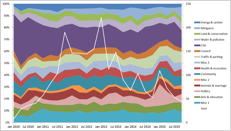
I modelled the whole corpus with 70 topics, which I grouped manually into eleven themes (I have since developed an automated method of grouping the topics, which I will describe later in this post). For the period 2000-2015, using six-month increments, and with the letters excluded, these themes are distributed as shown in Figure 2:
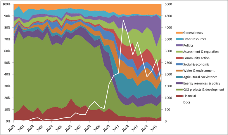
The results in Figure 2 are broadly consistent with what I found in my last post. The defining feature of this figure — of the whole corpus, really — is the dramatic shift in 2009-10 from discussion about CSG and LNG projects to discussion about the environmental, social, economic and political implications of CSG development. The corresponding graph for the letters is shown below. (If you’re viewing this on a desktop, this figure will flip to one shown in Figure 2 when you hover your mouse over it.) You’ll notice the gaping holes prior to 2008 — these reflect the almost complete absence of any letters in the corpus in this period.
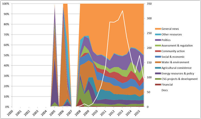
Figure 3. The 70-topic model applied to just the letters. Hover over the image to compare the letters with the other content in the corpus.
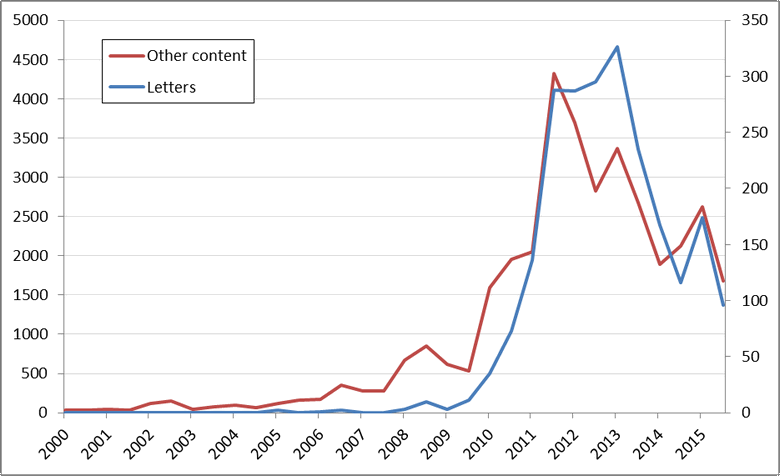
Ignoring the thematic content for the moment, we can see in Figure 4 how the volume of articles and letters compares over time. (Note that two separate scales are used, so the two datasets look to be of the same size, when in fact they are not.) While the two curves are broadly similar, there are some interesting differences. Although both rise quickly to a peak in 2011, the volume of letters initially lags behind the other content. Then, while the volume of other content falls, then letters continue to increase, peaking again in 2013 (I think this peak coincides with the Federal election). Both datasets then peak together in the lead-up to the New South Wales state election in 2015. Without looking closely at the data, my guess is that the sudden, late rise in the volume of letters is driven by the Lock the Gate campaign taking hold in Queensland and then New South Wales. The subsequent divergence from the other content suggests that the community was, at least for a time, more interested than the media in issues surrounding coal seam gas.
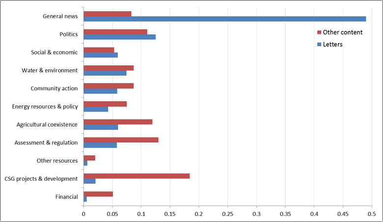
But the more striking difference between the letters and the other content is in the relative prominence of the themes. About half of the content in the letters is accounted for by topics that I classed as ‘general news’, a class that accounts for a relatively small slice of the other content. The other main difference is that the letters talk much less about financial matters, CSG projects and government regulation. The comparative thematic breakdown of the letters and the remainder of the corpus, minus the dimension of time, is shown more clearly in Figure 5.
A model just for the letters
An important methodological question that I’ll be grappling with as I move forward is how best to use topic modelling to compare corpora that differ significantly in their size and vocabulary. Put simply, the dilemma is that while using a single model will allow for direct comparisons between the corpora, it might not provide an accurate representation of the smaller corpus. On the other hand, using separate models will capture the topical structure of each corpus more accurately, but will make comparisons more difficult.
This consideration is what led me to split the corpus into two time periods in the previous post. In retrospect I think that decision might have been a bit dubious (I suspect I could have managed by increasing the number of topics instead), but in the case of the letters versus the remainder of the corpus, I think there is a stronger justification for using two separate models. Not only is the corpus of letters much smaller (17 times smaller, to be precise) and of a different language style, it also covers a wide variety of topics that barely feature in the rest of the corpus. Furthermore, these topics are distributed across the documents in a distinctive manner. While news articles tend to be about one topic at a time, most of the documents in the letters corpus are actually collections of letters (or text messages, or tweets, etc.), each from a different person and each about a different topic. And only one of the letters in a collection needs to mention coal seam gas in order for the whole collection to be included in the corpus. This is important because the way in which topics are distributed across documents is reflected in one of the parameters of the LDA algorithm (usually called alpha) that must be set by the user. The optimal value of this parameter is likely to be very different for the letters than for the rest of the corpus.
Anyway, the point is, in order to see what the letters are really about, I ran another topic model. Since the letters amount to a relatively small corpus, the time taken to process them with the LDA algorithm was fairly short — and by this I mean less than 10 minutes — even in R, which is much slower (but more flexible) than Knime. So I took the opportunity to experiment with the parameters and refine my workflow. One thing I found is that the results improved considerably (by which I mean the topics made more sense) as I increased the number of topics: at any rate, I found that 50 topics worked better than 40, and 60 topics worked better than 50. And picking up on an issue I was grappling with in my previous post, I also confirmed that removing the 25% of terms with the lowest average TF-IDF score did not undermine the power of the results.
Let’s get less thematical
I also used this process as an opportunity to develop a workflow in R that automatically clusters the LDA topics based on their degree of similarity to each other. My hope is that this will provide a quick and defensible alternative to manually classifying topics into higher order themes, which I find to be a time-consuming but essential step for dealing with large numbers of topics. To measure the similarity of each pair of topics, I used a metric called the Hellinger distance, which is designed for comparing probability distributions, which under the hood is what LDA topics actually are. The function to calculate this metric is included in the topicmodels package for R, so I assume it has some validity for this purpose. I then used R’s hclust function to group the topics into a hierarchy of similar clusters. The dendrogram that I used to cluster the 60 topics describing the letters is shown in Figure 6.
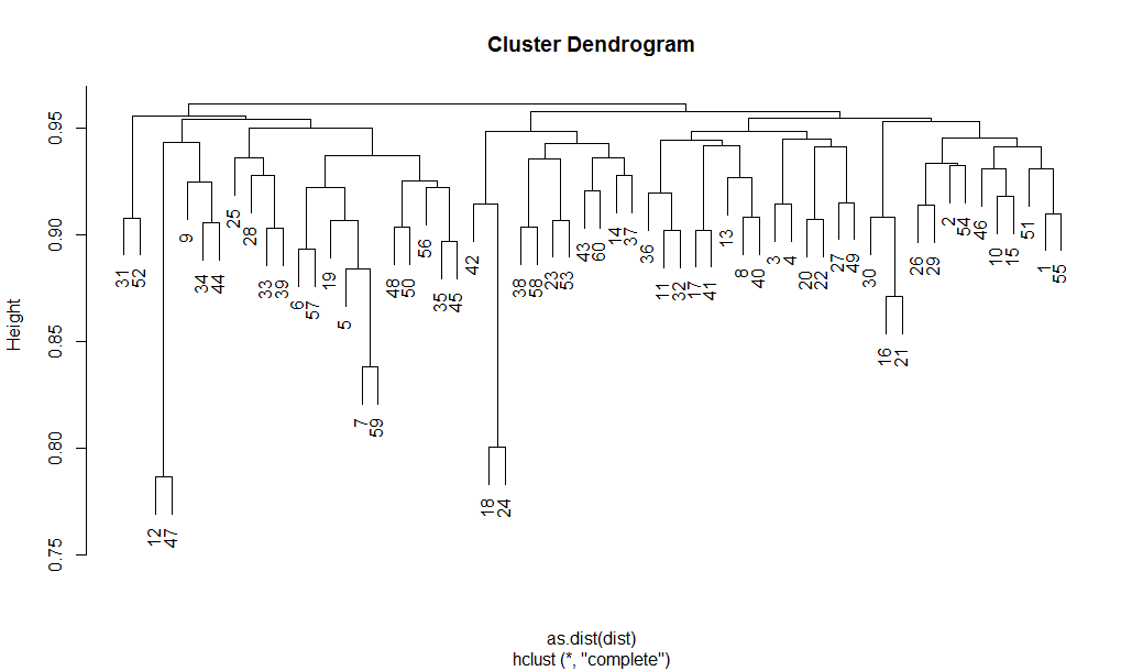
By specifying the number of clusters I want (using the cutree function), I can get R to assign each topic to a cluster. I also use the column order of the dendrogram to reorder the topic term outputs, which makes reviewing the topics much easier, even if the actual cluster divisions are not quite what I was hoping for.
So far though, the clusters assigned by this process tend to be pretty reasonable, especially when the topics themselves are subjectively satisfying. This apparent correlation between the success of the clustering and the success of the model is to me a very intriguing finding. In the example below, I can’t say that I would have grouped the topics in the same way as the clustering process did (I wouldn’t have thought to group animals with marriage, for example), but this might just be because my interpretation of the topics is biased in a way that the distance metric is not.
A picture of stability
Clustering the 60 topics into 15 groups using the method described above yielded the results in Figure 7. The timeline starts at 2010 because prior to then, there was not enough data to yield meaningful trends. The clusters, which I’ve tried to interpret as themes, are automatically generated, but the labels are my own. You’ll notice that there are three themes with the entirely unhelpful names of Misc 1, Misc 2 and Misc 3. These are clusters of topics in which I simply could not see a clear common thread. Misc 1, for example, includes topics about mental health, hospitals, drug abuse (so far so good), climate change and refugees (not so good). I could probably force these into separate clusters by moving further down the tree, but only at the expense of producing a more crowded, less intelligible graph.
The overall picture in Figure 7 is one of stability. There is no significant shift in the overall mix of themes. The most noticeable short-term spike is that in the Politics theme in the first half of 2015. This spike, which we’ve seen elsewhere several times now, coincides with the lead-up to the New South Wales state election. Otherwise, the plot is pretty boring, suggesting that overall, people talk about the same things over time.
You might also notice that the overall picture in Figure 7 is not one about coal seam gas. Most of the text in this corpus is about other matters, which is an inevitable result of multiple letters being included in most of the documents. The large theme that I have labelled ‘CSG’ includes 11 diverse topics, some admittedly much more clearly defined than others. Interestingly, the prominence of this theme actually decreases over time. Meanwhile, however, the theme I’ve labelled Metgasco increases in prominence, as shown below in Figure 8. The Metgasco theme contains just two topics, both of which relate to the activities of Metgasco in the Northern Rivers region of New South Wales.
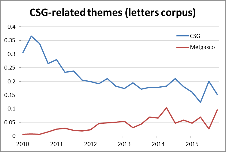
So, it looks as though discussion in the letters about topics relating to coal seam gas in a general sense has gradually declined, while interest in the activities the Northern Rivers region specifically has increased.
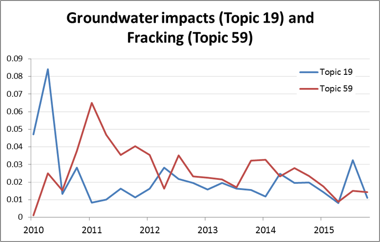
Digging further into the CSG theme, one interesting pair of topics that I noticed is that shown in Figure 9. Topic 19, which is about groundwater impacts, spikes early on and then drops to a much lower level, where it remains for the rest of the period. Topic 59, which is about fracking and the water contamination fears surrounding this technique, peaks about a year later than Topic 19 and then also declines, albeit at a slower rate. I suspect that the sudden interest in Fracking in 2011 was driven by the release of the movie Gasland.
Comparing corpora and topic models
I said earlier that I was interested in how best to use topic modelling to compare wildly differing corpora. Now that I’ve generated separate models for the letters and the broader corpus, let’s see how their outputs compare. In Figure 11 I’ve compared how the two models measure the prominence of similar topics within their native corpora. I need to stress that the topics being compared are similar, rather than identical. They have enough top terms in common that they could be reasonably interpreted to be ‘about’ the same thing, but they also contain differences that stem from the parameters of the models and/or the structure and vocabulary of the corpora. Two examples, corresponding with the groundwater and fracking topics in Figure 11, are shown here in Figure 10.
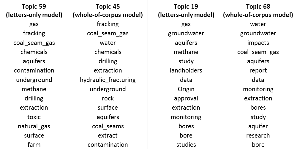
To be honest, I’m amazed at how similar the top terms of these topics are, given that they were generated with different parameters, corpora and software (the letters corpus was modelled with R, and the broader corpus was modelled with Knime). What I really should do is calculate the Hellinger distance between them, as I did in the clustering process discussed above, but that will have to wait. For now, their surface-level similarity gives me some confidence that any differences observed in their behaviour, such as those in Figure 11, are real rather than just mathematical artifacts.
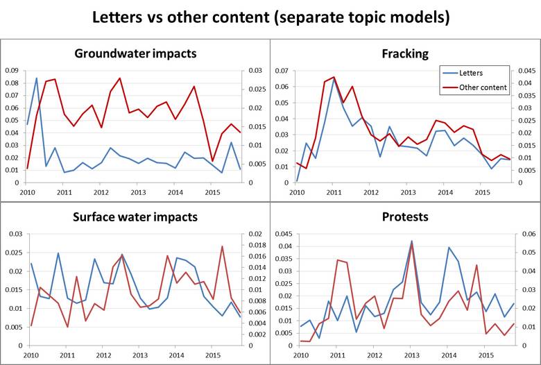
Figure 11 suggests that concern about fracking within the letters is almost perfectly in sync with the other news content. The same cannot be said for groundwater and surface water impacts, except perhaps for a period between 2012 and 2014 when there is some synchrony between the surface water topics. The protest topics show periods of difference as well as similarity.
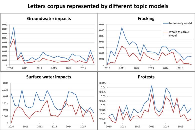
Figure 12 presents a different comparison. It shows how the two different models — one generated from the whole corpus, the other from the letters alone — measure the prominence of these similar-but-not-identical topics within only the letters corpus. These results provide further evidence of similarity between the two models. Except in the case of surface water impacts, the models follow one another closely, albeit with the whole-of-corpus model consistently tracking below the letters-only model. I’m only speculating here, but this gap might exist because the whole-of-corpus model is allocating some of the more idiosyncratic terms from the letters to one or more topics of their own — I’m thinking of the ‘marker topics’ that I used earlier to identify letters in the corpus.
Where are the letters coming from?
Despite my remarks at the beginning of this post about the importance of contextual information, I have proceeded to fixate on the content of the letters while saying nothing about where they came from or who published them. So I’ll finish with a small effort to correct this imbalance.
Figure 13 lists the fifteen publications with the greatest numbers of letters in the corpus. It also shows how much of the overall volume of letters and other content in the corpus each of these publications accounts for. For example, Lismore’s newspaper, the Northern Star, accounts for 27% of the letters in the corpus but only 3% of the other content (in absolute numbers, it accounts for about twice as many news articles than letters). The Northern Star also accounts for more than twice as many letters as any other source. Next on the list is the Northern Rivers Echo, which covers the region of Northern New South Wales in which Lismore is situated. The Richmond River Express, which is fourth on the list, is part of the same region. Between them, these three relatively small publications account for 40% of all the letters in the corpus. We knew this already, but clearly northern New South Wales is a hotspot of community interest in coal seam gas.
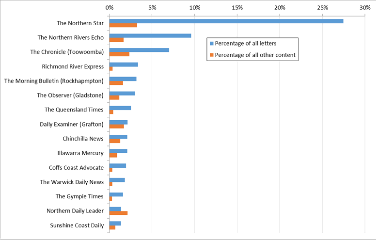
Figure 13. The 15 newspapers with the most letters in the corpus. The top few account for a disproportionate share of the letters in the corpus compared to other content.
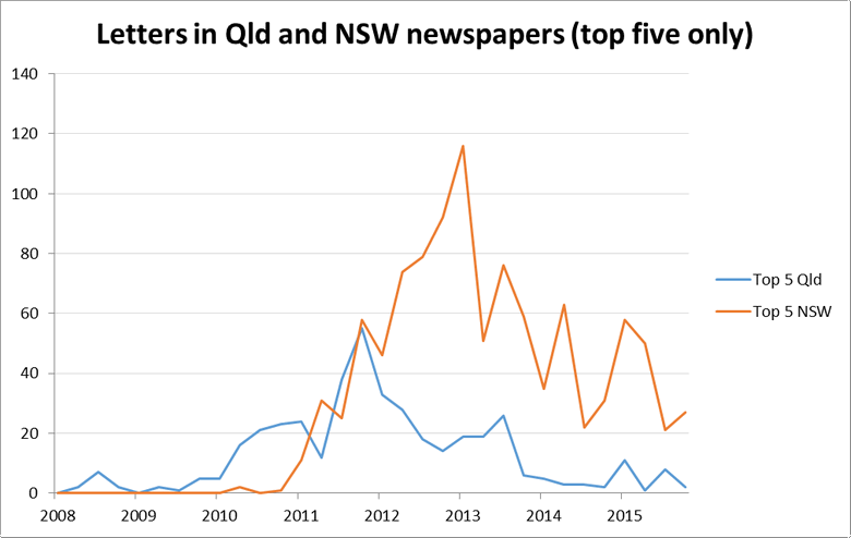
I’ll leave a more fulsome breakdown of the publications for another day 1, but will finish with one more teaser. Figure 14 charts the number of letters over time from the five newspapers from each state (that is, Queensland and New South Wales) with the most letters in the corpus. The overall magnitudes are interesting but not worth reading much into until they have been fleshed out with the complete set of newspapers. What I think is more noteworthy is the timing — specifically, the way the New South Wales publications peak well after the Queensland publications have begun to decline. This echoes a narrative I’ve started to weave from other threads of data, such as in the How the news moves post that I wrote way back in March.
Oh god I thought it would never end
I always start out meaning to make these posts short and snappy, I swear. But useful things start to emerge from them, and before I know it I have written 5,000 words. What were the useful things this time around? Pfff I don’t know, but it’s time for a glass of wine and some chocolate pudding.
Notes:
- May not actually happen ↩