My previous post was all about turning place names in news articles into dots on a map. Using a fairly straightforward method, I matched the place names in a collection of 26,863 news articles against the names and geographic coordinates in the Australian Gazetteer 2012, which lists and locates virtually every named place in Australia. Using such a comprehensive list created a fair amount of extra work, but resulted in a very rich and satisfying visualisation of how the news coverage about coal seam gas has moved over time. Ultimately however, I want to translate these rich visualisations into simpler narratives and numerical descriptions. And to do this, individual statistics for every one of the 1,448 places on my list will not be of much help. I will need some way of aggregating the locations into relevant regions or locales.

To achieve this, one could perhaps use some technique to group the locations based on spatial proximity — something akin to drawing fences around the places that form discrete clusters on the map. But there might be reasons besides proximity to group places together. Spatially distinct places might be united by common issues or events, just as proximate places might be subject to separate laws and controversies. Given that my ultimate object of study is public discourse, such non-geographical unifying factors may prove to be as important as geographical ones.

Latent Deary What?

Only some of these thoughts had crossed my mind when the idea hit me to use a topic modelling technique called Latent Dirichlet Allocation (LDA) to bring some order to my large list of locations. LDA is a technique that automatically identifies topics in large collections of documents, with a ‘topic’ in this context being defined as a set of words that tend to occur together in the documents that you are analysing. LDA uses some clever assumptions and iterative processes to find sets of words that, in most cases at least, correspond remarkably well with meaningful topics in the text. It is widely used for automated document categorisation and indexing, and more recently it has been applied to fields such as history and literary studies under the banner of the digital humanities. If you’re fluent in hieroglyphics, the Wikipedia page might be a good place to start if you want to know more about LDA. If you’re a mere mortal, pages like this one and this one offer a softer introduction.

Like many computational text analysis methods, LDA views each document as an unordered ‘bag of words’. (This might sound like the surest way to render a document meaningless, but the payoff is that it makes the text amenable to all kinds of statistical techniques.) So I figured, why not instead feed the LDA algorithm bags of places, which is exactly what I had created from my collection of news articles when preparing my last post. I saw no reason why LDA couldn’t turn this data into groups of locations that were both spatially and discursively meaningful. Places that are mentioned together in articles are likely to be physically close to one another, linked by social context, or most likely, both. Meaningful groupings of these places could be called geographic topics, or geotopics for short.

Using LDA to analyse geographical information is not entirely novel. One of the first things I ever read about LDA was Benjamin Schmidt’s highly instructive analysis of shipping logs. And a quick Google search reveals studies like this one, which adapts LDA to analyse geographical data in twitter streams. I’ve not yet come across an example where LDA has been applied to the outputs of named entity extraction (which I am doing here), but I wouldn’t be surprised to find one.

It’s also entirely possible that LDA is not the best tool to use for this purpose. There might be simpler statistical techniques that can do much the same thing, or different approaches that can do something better. But a large part of my motivation for this exercise is that I’m going to have to dabble in LDA sooner or later, and this is as good a way as any to start. Following Ben Schmidt’s lead, I figured that applying LDA to geographic data would be a great way to get a feel for how it works, at least at an intuitive level. And besides, if the experiment works, it could help to guide further analyses.

So does it work?

To cut the story short, yes it does work — and more effectively than I had dared to expect. Many of the LDA-generated geotopics matched specific areas where coal seam gas has been searched for, produced commercially, or debated by the community. Figure 1 shows two examples. Topic 7 corresponds with the Surat Basin gas fields in Queensland, while Topic 22 relates to the Pilliga Forest and Liverpool Plains region in New South Wales. The size of each circle represents the ‘weight’ that the location carries in defining the topic.

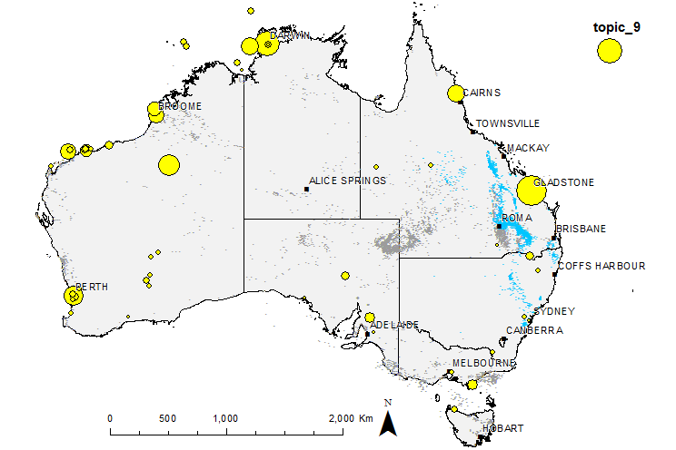
Some of the geotopics were less readily interpretable, bringing together widely scattered locations, such as in Figure 2. But in most of these cases, what looked at first like unrelated locations turned out to have a connection after all. For example, most of the prominent locations in Topic 9, including those in the ocean, are gas fields that have traditionally supplied the Australian LNG (liquefied natural gas) industry. The big exception is Gladstone, which is the export point for Queensland’s new CSG-to-LNG industry. The articles in which this geotopic is prominent tend to be about market conditions and investment tips.

However, even in cases where a geotopic offers a clear interpretation, things are not always straightforward. A closer look often raises questions about where the boundaries of a geotopic have been drawn. Why does the geotopic include some parts of a given region but not others? Is there a way to match one geotopic to a whole region, rather than having different topics describe separate parts?

How such boundaries get drawn changes depending on how you set certain LDA parameters. You need to specify, for example, how many topics you want the process to generate. There are also two variables, named alpha and beta, which control assumptions about the relative prominence (in other words, the distribution) of topics within documents and words within topics. Changing these variables can, I am told, dramatically alter the results that LDA produces.

When I plunged into my geo-LDA experiment, I didn’t have the patience to learn what alhpa and beta really meant, so I left them at the default values of the tool that I was using. I did, however, experiment with the number of topics, and I’ll report on the difference that this made later in this post.

The following sections get a bit nerdy. If you have no interest at all in the mechanics of LDA and what it does with geographic data, I suggest skipping to the regional roll-call.

Some technical details

A few words are in order regarding the particulars of how I produced what you will see in this post.

There are various implementations of LDA availble, including a program called MALLET and a package for the statistical analysis package, R. I’ll probably have to learn to use one of these if I want to do anything really clever with LDA, but for this initial experiment, I used the LDA module included in the data analytics platform Knime, which I have used to do much of my data wrangling and analysis thus far. This module is apparently itself an implementation of libraries within MALLET.

The Knime module provides a handful of parameters for the user to tweak. The most mysterious are called alpha and beta, which control assumptions about the distributions of topics across documents and words across topics. When I started experimenting with the module, I knew even less than this about these parameters, so I left them at their default values of 0.1 and 0.01 respectively. Since the results were so impressive, I never bothered to go back and change them. That’s an experiment for the future. ¹

Less mysterious were the parameters for the number of topics in the collection and the number of words per topic. I varied the number of topics from 15 to 30 to 50, and I’ll present some the results of that variation shortly. I played a bit with the number of words per topic, but found the results less interesting and eventually stuck with 50 words (i.e. locations).

Finally, there was the moderately mysterious ‘iterations’ parameter. I reduced this to 500 from the default of 1,000, based on a hunch (and nothing more) that because my documents were so simple (most of them consisted of just two or three place names) and the vocabulary so small (1,448 locations), I could afford to cut down on the amount of computation performed.

The data itself was the same set of 26,863 news articles as I have analysed previously, only this time I stripped the articles of all content except the place names that I had identified using the tagging procedure described in my last post.

Visualising each topic on a map was a simple matter of joining the topic definitions output table to the geographic layer I had prepared previously. The use of scalable circles to denote the locations worked perfectly here as well, because the LDA process assigns a weighting to every word (i.e. location) within a topic. So I used the size of the circle to indicate the weight of each location within the topic being viewed.

Spotting rogue locations – LDA as a diagnostic tool

As soon as I started to visualise the LDA outputs on a map, I discovered an unexpected side benefit of the process. It provided a fantastic way to diagnose mistakes I had made in preparing the data. As I described in the previous post, automatically matching place names to locations becomes tricky when you include names that could refer to more than one place, or that might refer to persons instead of places. The location tagging approach that I used allowed each name to match to only one location, and it could not reliably distinguish between persons and places. So I had to pick one location or another where multiple ones were possible, and I did my best to exclude any names that I felt were more likely to refer to people than locations. Inevitably, I made some omissions and sub-optimal choices in this process. Thankfully though, visualising the LDA geotopics makes these errors stick out like certain proverbial canine appendages. Do you notice something funny in this geotopic about the Hunter Valley, for example?

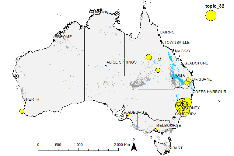
The vast majority of locations in this topic are in and around the Hunter Valley, just north of Sydney. But there are some obvious outliers. Let’s start with the trio of spots in the centre of Queensland. The most prominent of these is a parish (yes, a parish) by the name of Argus. Inconveniently, Argus is also the name of several regional newspapers, including the Hunter Valley’s Singleton Argus. The yellow spot to the south of Argus is another parish (I get the feeling I should not have included parishes in my tagging list), this one named Camberwell, which also happens to be the name of a village just near Singleton, as well as a suburb in Melbourne. The last of this trio of outliers is the town of Galilee, which shares its name not only with the underlying Galilee Basin, but also with the chief executive of the New South Wales Minerals Council.

Just next to Brisbane are two more outliers. One is the town of Moore, which features much less often in news about coal seam gas than Jess Moore, the spokesperson for Stop CSG Illawarra, or Clover Moore, the Mayor of Sydney. The other is Drayton, an outer suburb of Toowoomba — and the name of an iconic winery in the Hunter Valley, as well as a nearby coal mine.

Many of the geotopics that I inspected included outliers like these, most of which I will need to remove from my tagging list or assigned to different locations for mapping purposes. Without visualising these LDA outputs, however, I don’t know how or when I would have found them. Thanks to this exercise, I now have a long list of corrections to make to my data. Note, however, that the remainder of this post uses the uncorrected data. Where the errors produce misleading results, I’ll point them out.

I’m not quite done with Topic 32 in Figure 3. In the discussion above, I ignored the yellow spot near Adelaide, and the one south of Perth. These are more interesting than the other outliers, because they are not errors. They are exactly where they should be. They denote the Margaret River and the Barossa Valley, both of which are important wine-making areas that happen to be close to prospective gas fields. The LDA process has lumped them together with the Hunter Valley locations because news articles about gas developments in the Hunter Valley frequently cite them as areas where analogous policy debates and community campaigns are taking place. This is a perfect demonstration of how these geotopics embody both geographic and discursive associations. Whether this is a good thing or not depends entirely on how you wish to use them.

How topic number affects topic content

As I mentioned earlier, one of the parameters that you need to specify with each LDA run is how many topics you want to discover. A logical question to ask is how the number of topics affects the composition of the topics themselves. Do the topics become more specific as their number increases? And what does this mean when the topics are composed of locations rather than concepts?

Based on my observations, some of which I will share below, the topics do indeed become more specific as you generate more of them. And in most cases, the more specific geotopics do represent meaningful geographic divisions, although sometimes the meaning doesn’t become clear until the discursive context is considered — and even then, there are cases where it is hard to see why one topic has been split from another.

To explore the relationship between topic number and topic content, I compared the results that were generated when the number of topics was set to 15, 30 and 50. In each case, I asked the algorithm for 50 words per topic (in retrospect, I probably should have scaled the number of words inversely to the number of topics, but anyway). My eventual conclusion was that more topics is generally better, though I suspect that there will usually be a point of diminishing and then negative returns. More importantly though, this exercise suggests that the optimal number of topics may depend on the specific questions that you want to answer, as some questions will call for higher levels of topical aggregation than others.

This should all make more sense when you see the examples below, which explore the geotopics relating to the Surat Basin and Darling Downs region in Queensland.

A case study – the Surat Basin and Darling Downs

The coal seams of the Surat Basin in Queensland were not developed intensively until around 2007, when local gas producers began to fix their sights on the global export market. The development of these coal seams brought the industry into contact with the high-value farming areas of the Darling Downs, and especially the Western Downs Region, which stretches roughly from Dalby to Wandoan, taking in the towns of Chinchilla, Miles and Tara. A range of conflicts and controversies ensued, and attracted a large amount of news coverage, as the visualisations in the previous post demonstrate.

The high number of articles about this region meant that the LDA algorithm had a lot of data to work with in generating relevant geotopics. The 50-topic run produced at least seven separate geotopics relating in some way to the Surat Basin and Darling Downs. The most comprehensive of these geotopics, which the algorithm designated as Topic 7, is shown below in Figure 4. This geotopic includes nearly all of the gas fields in the region, with the exception of the fields between Roma and Wandoan, as well as a large field further north of Roma.

This geotopic has clear analogues in the 15-topic and 30-topic runs. You can see the analogous topic from the 15-topic run by hovering your mouse cursor over Figure 4. Ignoring the obvious difference in marker weights, the overall coverage and distribution is very similar, though each geotopic seems to have its own set of lightly weighted locations.

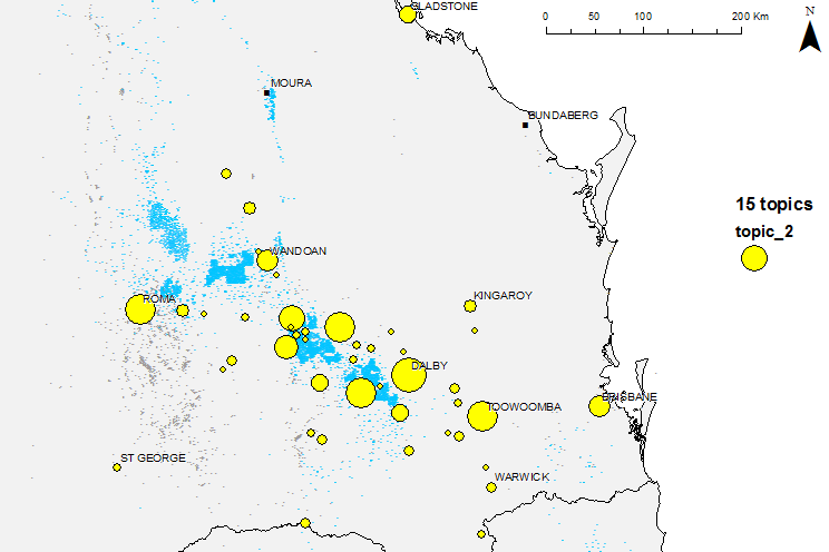
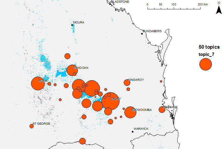
Figure 4. Topic 7 from the 50-topic run covers most of the CSG producing areas in the Surat Basin in Queensland. Hovering over the image reveals an analogous geotopic from the 15-topic run.

Each of the runs also generated geptopics that covered a more specific part of the Darling Downs region. Figure 5 show an example from the 15-topic run. Compared with the more comprehensive geotopic, this one focusses more on Chinchilla and Tara, and less on Dalby and other places to the east. This geotopic has an analogue in the 30-topic run, which you can see by hovering over Figure 5. To my eye, the 30-topic version is noticeably more dense and focussed than the 15-topic version — a relationship that I observed in nearly every instance of analogous geotopics. Presumably, this occurs because a lower number of topics forces each topic to be more general, thus bringing in locations that are more distant from the main cluster. (If I had allowed more words per topic in the 15-topic run, perhaps this difference would diminish.)

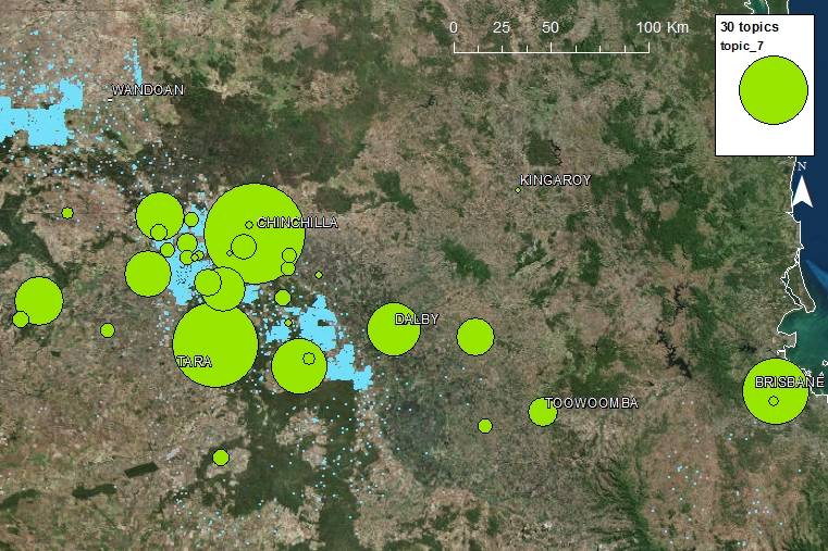
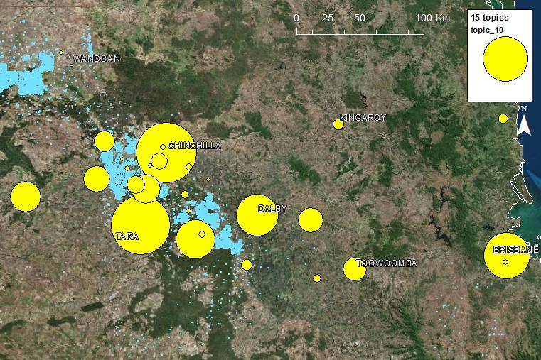
Figure 5. Topic 10 from the 15-topic run emphasises locations around Chinchilla and Tara. Hovering over the image reveals an analogous geotopic from the 30-topic run.

In the 50-topic run, there is no single geotopic that is closely analogous to those in Figure 5. Rather, there are several more specific topics that cover or emphasise separate areas. For example, Topic 25 in Figure 6 emphasises the western end of the geotopic above, while Topic 20 (visible when you hover over Figure 6) emphasises the central portion. ²

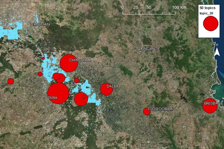
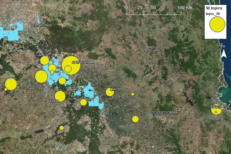
Figure 6. Topic 25 and Topic 20 (visible when you hover over the image) emphasise subtly different areas within the Western Downs.

Topic 48, visible when you hover over Figure 7, provides yet another subdivision of the Western Downs, this time emphasising the areas to the south and west of Dalby (these were hardly represented at all in the topics in Figure 6, but were in the more comprehensive topic in Figure 4).

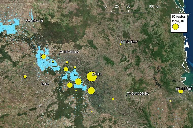
Figure 7. Topic 48 (visible when you hover over the image) emphasises yet another part of the Western Downs region.

Why did the 50-topic run produce not one, but three separate geotopics covering the Western Downs? What does each of these geotopics ‘mean’? To interpret these and other ambiguous geotopics, I inspected the articles in which they are most prominent (this is something that the LDA outputs make very easy) and looked for a common theme that might unite the locations. I also plotted the relative prominence of the geotopics over time, ³ looking for trends and peaks that might relate to events in the news coverage.

My conclusion is that these three geotopics are divided according to two main factors — the acreages of the different gas companies, and the issues and conflicts that are specific to these acreages.

The gas tenements in this region are operated by four CSG producers — Santos, Arrow Energy, Queensland Gas Company (QGC), and Origin Energy. Although in some places the tenements of the different companies get a bit tangled up with one another, in general they occupy distinct areas. Santos operates in the fields to the south and north of Roma.

Origin and QGC both operate in the area to the west and south-west of Chinchilla, and QGC also has tenements further south between Dalby and Tara. These are the areas emphasised in Topics 20 and 25. The articles relating to Topic 20 are largely about QGC and the conflicts with the community around Tara, particularly in early 2011 when the Lock the Gate Alliance became active. This is consistent with the peak in the relative prominence of Topic 20 in the first quarter of 2001, shown in Figure 8.

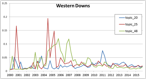
QCG and Tara also feature in many articles about Topic 25, but these articles tend focus on a slightly earlier time period and include more coverage of Origin’s activities and the suspicious bubbling of the Condamine River, which was first reported in mid-2012. At least, that’s what I inferred from reading the articles that scored most highly with this topic. The temporal analysis in Figure 8 suggests instead that this topic might have something to do with events in 2004 and 2005. The peaks in this topic in those years correspond with energy supply deals involving Origin, QGC and a company with premises on Gibson Island near Brisbane.

Arrow Energy operates mainly along the western fringe of the Condamine floodplain, to the west and south-west of Dalby. Not surprisingly, Arrow features heavily in the articles in which Topic 48 (Figure 7) is dominant, as does QGC, which operates fields not far from Arrow’s tenements. The peaks in prominence of Topic 48 between 2004 and 2007 (Figure 8) correspond with reports of energy supply deals specific to these areas struck by these two companies.

Are these divisions useful? To be honest, I’m not sure. In most cases, I think I would happily trade these three vaguely divided geotopics for a single consolidated Western Downs geotopic, although it’s fair to say that neither the 15-topic run nor the 30-topic run fully achieved this either (the topics in Figure 5 come close, but they under-represent the Arrow Energy areas included in Topic 48). Separating the acreages of the different gas companies could be useful, but these geotopics didn’t do a great job of that either. Knowing that issues such as the conflicts at Tara and the bubbling of the Condamine River are discursively separated is interesting, but hardly surprising, and this distinction is likely to be more apparent when LDA is put to its more traditional purpose of analysing the semantic content of the data.

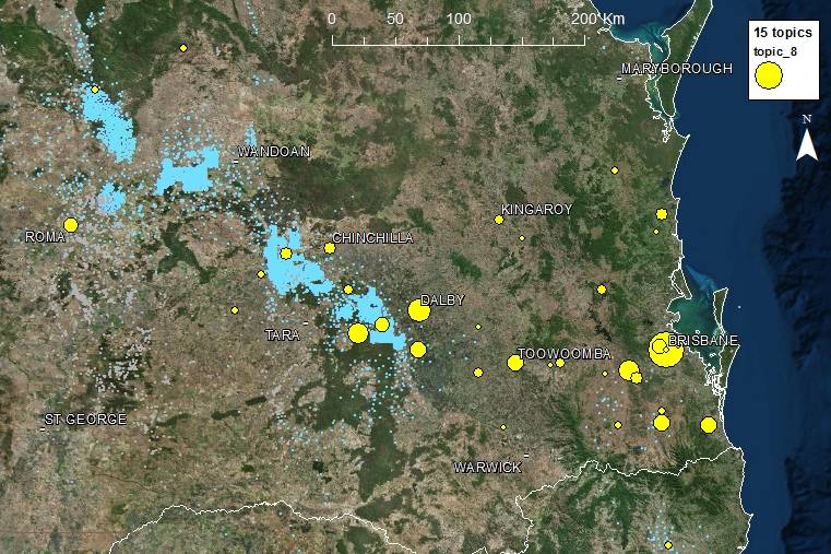
But there’s still more! The 50-topic run produced two further geotopics covering the Darling Downs. The one shown in Figure 9 is more focussed on the region between Toowoomba and Dalby. The articles that feature this topic date mostly from before 2011, and are as much about coal mines as coal seam gas. They feature groups such as the Central Downs Irrigators, the Basin Sustainability Alliance, and Freinds of Felton, which became less prominent once Lock the Gate got going. So this geotopic is interesting because it points to a distinctive chapter in the public discourse on coal seam gas. But again, perhaps this chapter would be more easily identified by analysing the full contents of the articles rather than just the locations.

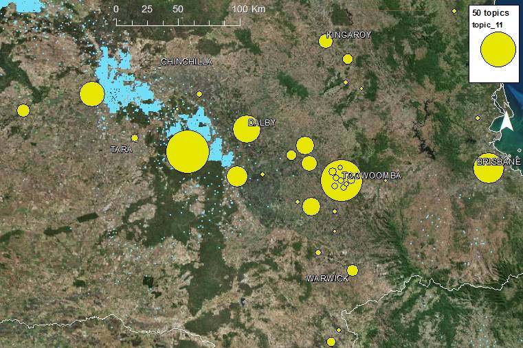
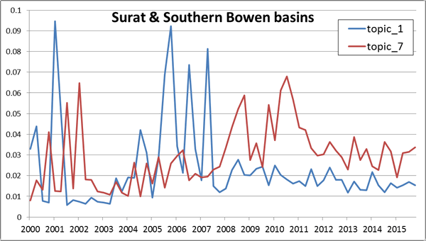
Topic 1 in Figure 10 fills a gap left by all of the Surat Basin geotopics discussed so far. It is the only one in the 50-topic run that includes the gas fields to the north of Roma — these being Fairview and Spring Gully — as well as locations to the east of Roma, including the gas hub Wallumbilla. The separation of these gas fields from those in the other topics is appropriate, given that they in fact tap into the southern Bowen Basin rather than the Surat, and were developed earlier than most of the Surat Basin fields — a difference reflected by the peaks in Topic 1 between 2005 and 2007 in Figure 11. Another point of interest in Figure 11 is the peaks in Topic 7 between 2000 and 2003. These coincide with reports of the first CSG pilot projects in the Surat Basin, operated by QGC and Arrow.

Topic 1 also has an added surprise, which I’ll reveal in the next section.

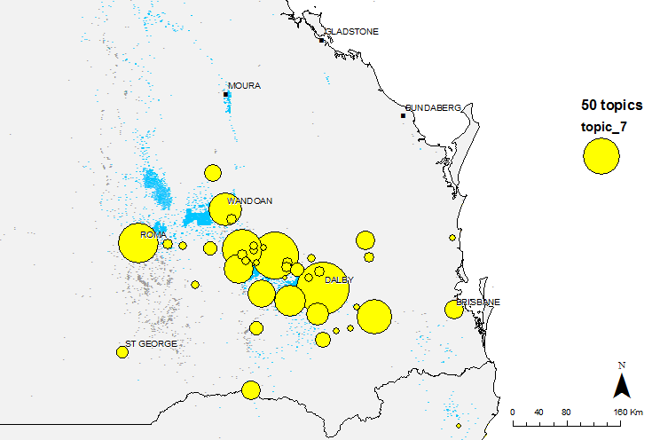
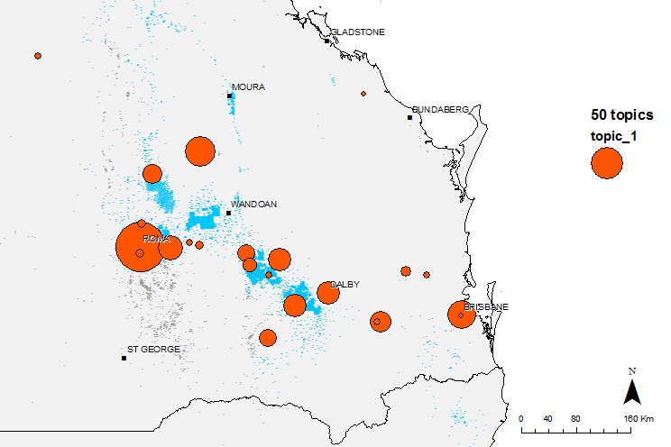
Figure 10. Topic 1 emphasises Roma and the nearby gas fields, thus filling the gap left by Topic 7 (visible upon hovering over the image).

 

Combos and chimeras

A common occurrence in the 15-topic and 30-topic runs was the joining of two seemingly unrelated areas within the same geotopic. The geotopic in Figure 12 is a good example. It combines elements of the Dalby-focussed Topic 48 (Figure 7) with what in the other runs is a separate topic for the Scenic Rim area south of Brisbane (see the regional roll-call below).

Another example is Topic 10 from the 15-topic run, only part of which was shown earlier in Figure 5. That topic also includes a cluster of locations to the north and west of Hobart (the Southern Midlands, I think this region is called), where a company called Petratherm was granted a licence to explore for shale oil and gas (not the same as CSG, but involving the use of fracking) in 2014. This cluster might warrant its own geotopic, but it was not separated even in the 50-topic run, which combined it with a hodge-podge topic covering various gas-producing regions around the country.

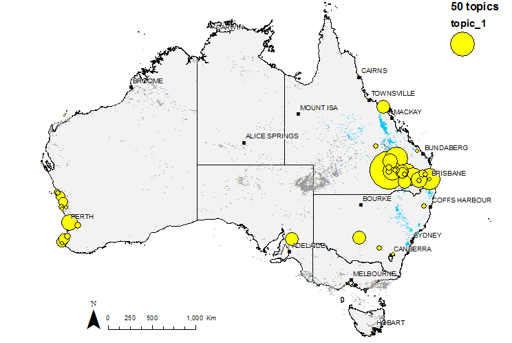
Another region that the 50-topic run failed to separate is the area on the West Australian coast north and south of Perth. This region was lumped together in Topic 1 with locations in the Surat and southern Bowen basins, as shown in Figure 13. I examine this region more closely in the regional roll call below. The question that arises here is how many topics need to be generated before regions like these are allocated topics of their own?

Some geotopics look like chimeras but are in fact united by a theme. The topic in Figure 14, for instance, joins together several gas-producing regions as well as the port city of Gladstone. The common thread is the pipeline corridor through which coal seam gas is taken to Gladstone to be liquefied and exported, and which was the subject of a large handful of news articles in the dataset.

Regional roll call

Whatever the technical and theoretical explorations above amount to, the fact remains that the LDA analysis successfully identified a long list of meaningful groupings of locations around which further analyses of news and other public discourse could be structured. Essentially, the process produced a roll call of regions and locales that have been the subject of more or less separate discussions about coal seam gas. Prior to this exercise, I was not even aware that coal seam gas was being debated in some of these areas.

I discuss each region in turn below (except for the Surat Basin and Darling Downs, which I discussed above). I make no claim to this list being definitive or comprehensive. It’s entirely possible that a tweak of the LDA settings would split the geotopics differently, or even identify entirely new groupings. If you know of any other regions that could be included here, feel free to leave a comment. All of the geotopics discussed here are from the 50-topic run.

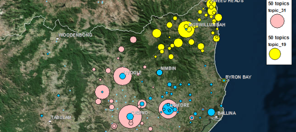
The Northern Rivers

From 2011 onwards, the Northern Rivers region in New South Wales became a hotspot for community opposition to coal seam gas, and generated a large amount of news coverage (see the previous post for visual evidence of this). The high number of news articles discussing this region presumably helps to account for the rich assortment of geotopics that the LDA process generated to describe it. In the valleys between Tweed Heads and Ballina, the 50-topic run identified four distinctive geotopics, all of which are shown in Figure 15. Topic 19 clearly relates to the Tweed Valley, while the other three all pivot around the city of Lismore. Topic 31 focusses on Metgasco’s tenements between Casino and Kyogle, which was the frontline of the Battle for Bentley (warning: stirring video). Topic 23 includes some of these locations but also incorporates a smattering of localities nearer to Lismore. Finally, Topic 29 emphasises locations along the coast, including Ballina and Byron Bay.

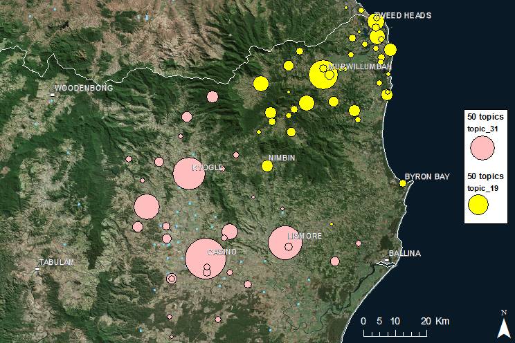
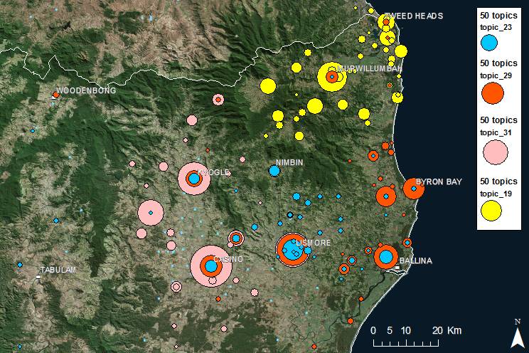
Figure 15. Four geotopics emphasising different parts of the Northern Rivers region, namely the Tweed Valley (Topic 19), Casino and Kyogle (Topic 31), Lismore (Topic 23), and Byron Bay (Topic 31). Hovering over the image removes topics 23 and 29.

The Lismore and Casino/Kyogle geotopics are charted over time in Figure 16, along with Topic 49, which relates to Grafton and the Clarence Valley. As Figure 17 shows, Topic 49 also incorporates locations as far south as Coffs Harbor, which is part of the Mid North Coast rather than the Northern Rivers. Coverage of all three of these geotopics began to rise in 2011, I suspect as a result of Lock the Gate becoming more active. But the more dramatic rise came in 2012, with the Lismore geotopic jumping about eight months ahead of Casino and Grafton. The early rise in the Lismore topic, I suspect, reflects the mobilisation of the local community, as this topic includes many of the populated places in the region. The sudden peak in Topic 31 (Casino and Kyogle) at the start of 2013 coincides with a blockade of Metgasco’s exploration activities at Glenugie (warning: autoplay video), which by the end of January had moved to Doubtful Creek. The spike in Topic 23 at the end of 2014 appears to relate to the New South Wales Government’s enforcement of its suspension of Metgasco’s exploration licence at Bentley.

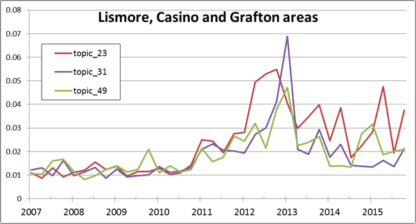
Figure 16. The relative prominence over time of geotopics relating to the areas around Lismore (Topic 23), Casino (Topic 31) and Grafton (Topic 49).

 

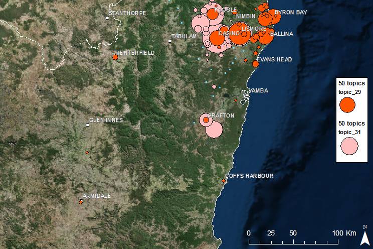
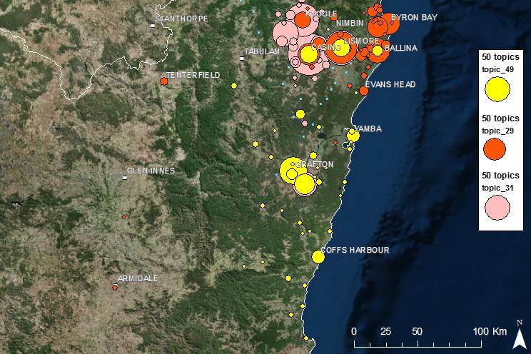
Figure 17. Topic 49, shown here with two of the other Northern Rivers geotopics, relates to the Grafton region. Hovering over the image removes Topic 49 to show the overlap with the others.

Sydney and surrounds

Up here in Queensland, it’s easy to believe that coal seam gas has never been produced anywhere else, but it has in fact been produced commercially in Camden, south-west of Sydney, since 2001. Two geotopics relate to this project, both shown in Figure 18. Topic 37 incorporates some locations beyond Camden, such as the Blue Mountains, while Topic 33 is focussed more tightly on the project area, and especially locations relevant to a proposed (but then abandoned) northern expansion of the project.

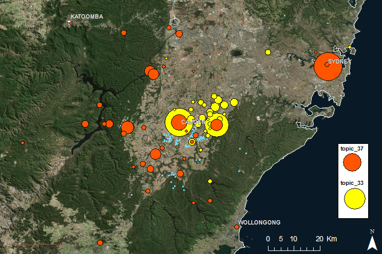
Figure 19 shows the history of these two geotopics. The peaks between 2000 and 2002, although representing only a few news articles, relate to the commencement of commercial operations. The spike in both topics in 2006 relates to coverage a takeover bid on Sydney Gas by QGC, and the spike in 2013 in Topic 33 relates to the proposed northern expansion.

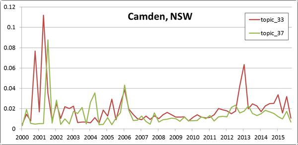
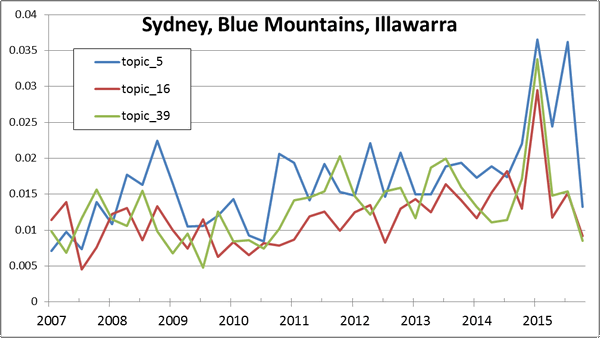
Figure 20 shows three more geotopics relating to the greater Sydney area. The tightest is Topic 39, which captures Wollongong and the Illawarra region. Although very few gas wells have been drilled in this area, it is the focus of a dedicated Stop CSG Illawarra campaign. Topic 16 relates to the Hawkesbury, Blacktown and Blue Mountains areas. Environmental groups from these regions formed an alliance in 2013 to protect Sydney’s water supply from risks associated with gas development. Finally, Topic 5 incorporates locations across a broad area, including metropolitan Sydney, the Central Coast (around Gosford), Wollongong and Camden. I’m not sure what unites these locations, but several of the articles relating to this topic mention that the gas exploration licence PEL 2 covered much of the area from the Central Coast to the Illawarra region.

The cancellation of PEL 2 in July 2015 corresponds with the final peak in Topic 5 in the graph in Figure 21. The peak in all three topics in early 2015 is probably related to the lead-up to the New South Wales state election, held in March 2015.

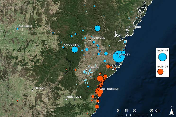
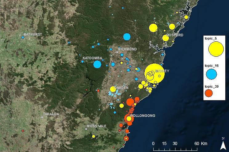
Figure 20. Geotopics relating to the Blue Mountains (Topic 16), the Central Coast (Topic 5) and the Illawarra region (Topic 39). Hovering over the image removes Topic 5.

Gloucester and the Hunter Valley

Figure 22 shows two more hotspots of community action against coal seam gas. Gloucester (Topics 17 and 30) in particular became a flashpoint in recent years, until AGL pulled out of its operations there in February 2016. Of the two Gloucester-related geotopics, Topic 30 is clearly the most targeted, while Topic 17 takes in more of the surrounding region.

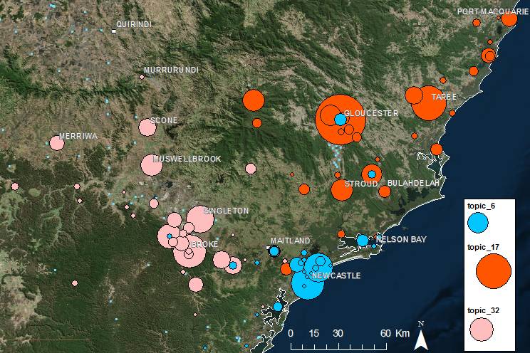
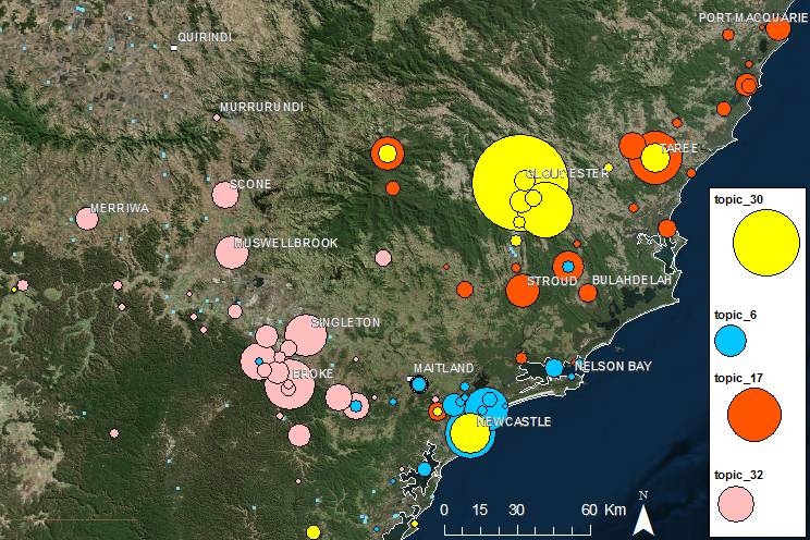
Figure 22. Four geotopics relating to the Hunter Valley and Gloucester regions. Hovering over the image removes Topic 30.

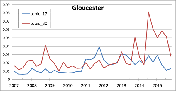
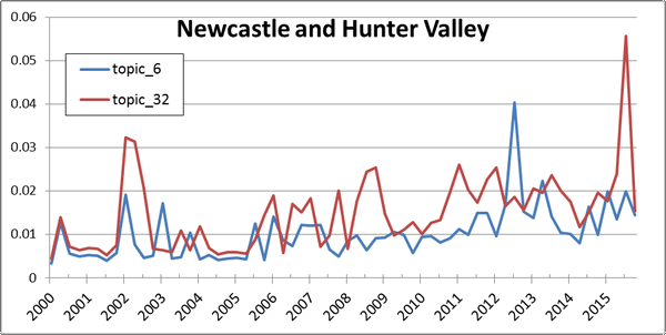
Figure 23 shows that the two geotopics have behaved quite differently over time, with Topic 30 proving to be the most dynamic. The spike in Topic 30 in late 2008 relates to the sale of the project by QGC to AGL, while the slightly larger spike in late 2013 coincides with debate about AGL’s proposal to irrigate with CSG water on the Avon River floodplain. The really big jump in the second half of 2014 can be attributed to several events. One is the release of a report from the Chief Scientist and Engineer of New South Wales recommending additional research into the vulnerability of groundwater systems like the one underlying Gloucester. Meanwhile, the government was proposing to fast-track approvals for AGL to frack in the area. In August 2014, the state renewed AGL’s petroleum exploration licence. Soon afterwards, there were revelations of undisclosed political donations from AGL while the approval was pending. No wonder this development became controversial!

Communities in the Hunter Valley — the focus of Topic 32 — have been mobilising against gas development there since at least 2006, and they too had reason to celebrate when AGL pulled out of the region in July 2015. As far as I know, a similar backdown is still forthcoming from the holders of the exploration licences round Fullerton Cove and Newcastle (Topic 6), which the local community campaigned against in 2012 and 2013.

The Pilliga Forest and Liverpool Plains

While AGL and Metgasco are revising down their ambitions for gas development in New South Wales, Santos appears to remain committed to progressing its exploration and appraisal program at Narrabri and the Pilliga Forest, captured in Topics 44 and 47. Meanwhile, activists buoyed by their success elsewhere in the state are pledging to shift their energies towards stopping this project.

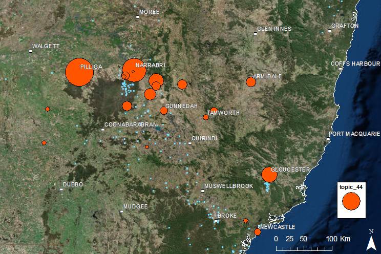
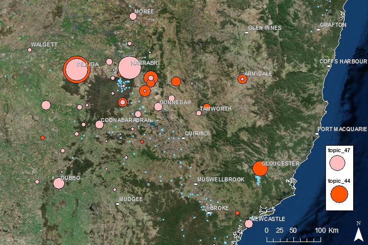
Figure 25. Two geotopics pertaining to the Pilliga Forest and Narrabri.

I’m not entirely sure what to make of the two geotopics in Figure 25. The circles over the town of Pilliga are visually misleading, as they are mostly picking up references to the Pilliga Forest. But even leaving that gripe aside, the locations in these topics are quite scattered, and it’s hard to know how to interpret them. I suspect that this is partly because the region is sparsely populated, so there are fewer references in the news to community meetings and demonstrations close to the project areas. Indeed, much of the coordinating action seems to take place in Armidale, which is a long way from the gas fields. As for the southern extent of Topic 47, a look at the source articles suggests that it relates to reporting of an exploration licence south of the Pilliga, extending as far as Dubbo and Lithgo, that was refused by the New South Wales Government in April 2014.

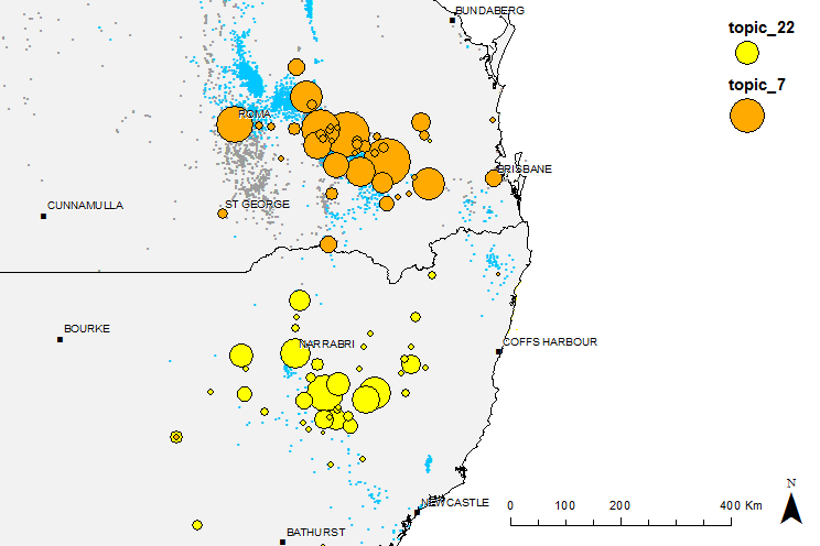
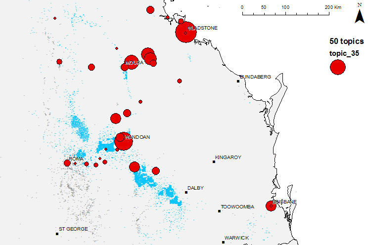
Two more geotopics relevant to this region are shown in Figure 26. Topic 22 includes the Pilliga Forest but focuses more on the Liverpool Plains, where Santos previously ran a pilot project at Spring Ridge. Topic 36 is an odd one, until you realise that it relates to proposals for a Narrabri to Newcastle gas pipeline, which would have supplied an LNG terminal at Newcastle. This is the cousin to Topic 35, which, as discussed earlier, relates to the pipeline delivering CSG from the Surat Basin to Gladstone.

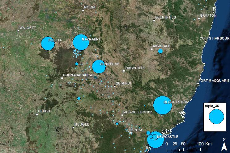
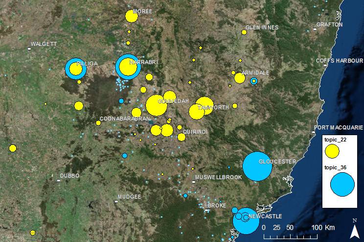
Figure 26. Topic 22 includes the Pilliga Forest but is primarily about the Liverpool Plains south of Gunnedah. Topic 36 relates to a proposed gas pipeline from Narrabri to Newcastle.

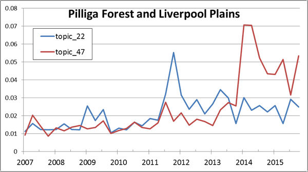
Figure 27 shows the relative prominence of the Pilliga Forest and Liverpool Plains geotopics. The blip in Topic 22 in 2009 appears to relate to Eastern Star’s successful drilling at Narrabri. The much bigger spike in late 2011 coincides with a community blockade in the Liverpool Plains, and the unlikely entrance of shock-jock Alan Jones into the CSG-versus-farming debate. While Topic 22 subsequently settles down, Topic 47 erupts in 2014, initially in response to a small spill of CSG water at Santos’ pilot project in the Pilliga Forest.

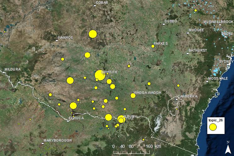
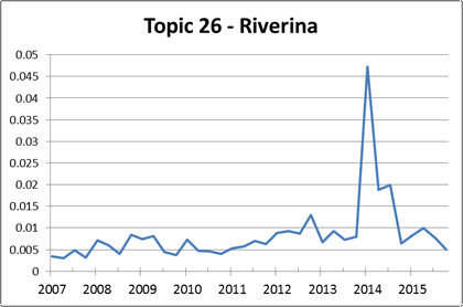
The Riverina

I had no idea that this agricultural region was caught up in the coal seam gas boom. Indeed, the New South Wales Government’s database shows but a single gas well, located about 50km south of Griffith. That well was drilled in 2003, but more recent controversy stems from an application by Grainger Energy for an exploration licence in late 2013. This application was apparently rejected in March 2014, but the community remained wary of further applications. The level of coverage of this region in early 2014 (visible in Figure 29) was no doubt further increased by the involvement of Lock the Gate.

Wide Bay and the Scenic Rim

Returning to Queensland now, the two geotopics in Figure 30 relate to regions north and south of Brisbane. Topic 21 could, at a stretch, be interpreted as a geotopic for the Scenic Rim region. Arrow Energy has been exploring in this region since at least 2005, but the community had well and truly turned against them by 2012. Even Campbell Newman said he didn’t want them there, though admittedly he was trying to get elected at the time. In any case, Arrow walked away from the region in May 2015.

Topic 40 (visible when you hover over the image) also includes the Scenic Rim, but focusses more on coal mining activities between Brisbane and Toowoomba. The presence of this coal-based geotopic among news articles discussing coal seam gas is a reminder that these two separate industries are sometimes discussed in conjunction with one another.

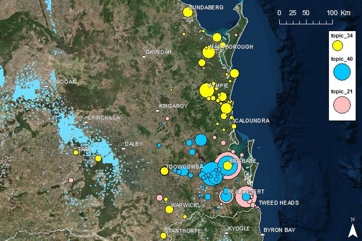
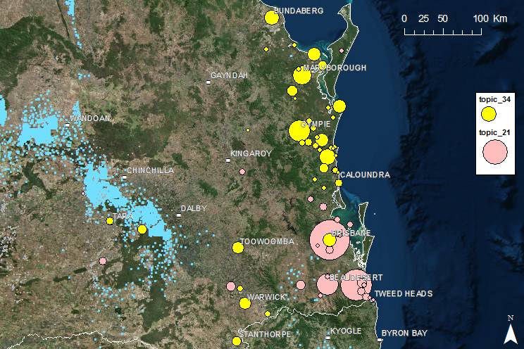
Figure 30. Three geotopics in the region around Brisbane. Topic 21 includes the Scenic Rim area, but is heavily weighted towards Brisbane. Topic 40, meanwhile, is weighted towards Ipswich and relates more to coal mining than to coal seam gas. Topic 34 captures the Wide Bay region.

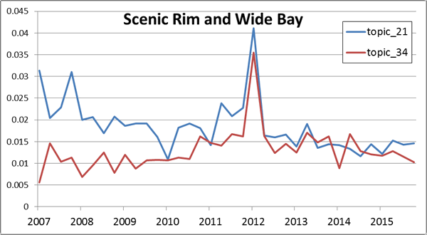
Topic 34 corresponds with the Wide Bay region, which is another place where I didn’t even know CSG exploration was happening. Apparently though, it’s been going on since around 2007. There’s not much that can be reliably inferred from the graph in Figure 31 except for the very strong spike in both topics in the lead-up to the March 2012 Queensland election.

Central and Northern Queensland

The gas fields of Moranbah and Moura in Central Queensland are where the coal seam gas industry in Australia began, way back in 1996. Topic 15 does a good job of catching these two areas (there is no topic that captures only one or the other), along with the regional centres along the coast (though Bowen is mostly picking up references to the Bowen Basin). The sparsely populated Topic 13 has more of an emphasis on the exploration areas of the Galilee Basin, near Longreach. (The biggest dot is for the town of Galilee, but this is in fact fed by references in the text to the Galilee Basin.) The sparsity of this topic probably reflects the small amount of news coverage that gas exploration in this area has received.

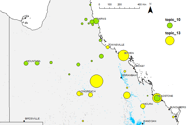
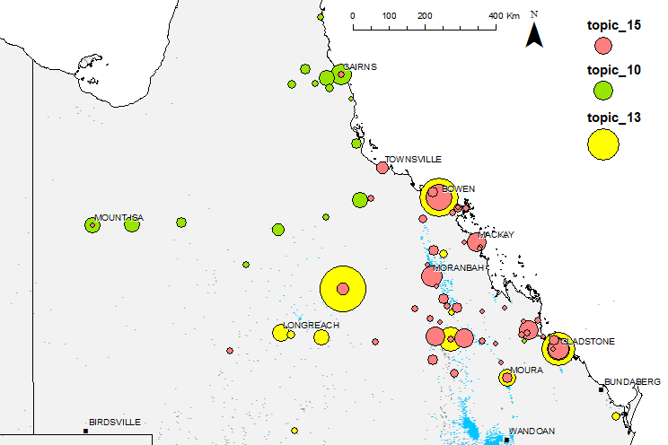
Figure 32. Three geotopics in central and northern Queensland, focussing on Moranbah and Moura (Topic 15), the Galilee Basin  (Topic 13) and northern Queensland (Topic 10).

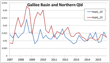
Gas exploration further north in the Galilee Basin is what unites some of the locations south-west of Townsville in Topic 10. The cluster of locations west of Cairns relate to gas exploration by the Mantle Mining Corporation at Mount Mulligan, the site of one of Australia’s worst ever mining disasters. This exploration permit was surrendered in April 2015. There are so few articles discussing these areas that the timeseries data in Figure 33 is next to useless. I managed to verify, however, that the peak in Topic 13 in 2008 relates to AGL’s announcement of its pilot program in the Galilee.

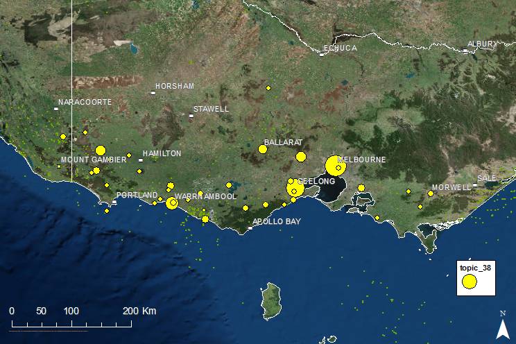
South-west Victoria

This is an other region that was not previously on my radar. It appears to be one area where the Lock the Gate campaign jumped in before any gas exploration had even started, in late 2011. Interestingly, the relative prominence of this topic (Figure 34) did not increase in response to this development. The Victorian Government has since placed a moratorium on unconventional gas exploration (there are possible shale oil and tight gas reserves here in addition to coal seam gas) and fracking. However, it appears that the community will remain on high alert until the ban is made permanent.

South-western Western Australia

As I mentioned earlier, the LDA algorithm actually lumped the cluster of locations in Figure 35 together with an unrelated cluster of locations in Queensland. So the settings may need to be tweaked (or the data expanded) to force this into its own geotopic. From what I can tell, the majority of potential unconventional gas resources in Western Australia are in the form of tight gas or shale gas. Coal seam gas is the minor player here, but fracking is the common thread. Several companies have apparently prospected in the region in Figure 35 (which for reasons that I do not understand is called the Mid West), though to what outcome I am not sure. Fracking has also occurred as recently as September 2015 in the Kimberley Region.

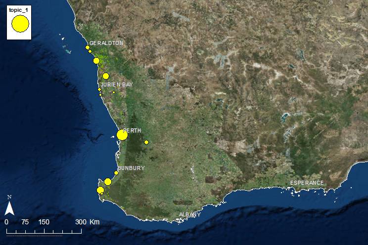
Figure 35. This cluster of locations on the West Australian coast is actually part of a geotopic that pertains primarily to the Surat Basin in Queensland.

So… what just happened?

At one level, I just used a very complicated method — applying LDA to extracted named entities and mapping the results — to learn something relatively simple, namely, the places in Australia where coal seam gas has been controversial. I probably could have gleaned this information through other means, such as by browsing the member groups of the Lock the Gate Alliance. However, I would not have learned much about the news data that I ultimately want to analyse. Nor would I have learned what I have about the LDA process itself, some of which I might not have learned as easily had I only applied LDA in the more conventional way.

An important thing to remember is that while the geotopics discovered in this exercise might sometimes correspond with how coal seam gas development and community responses have unfolded ‘on the ground’, ultimately they only reveal how the geography of these phenomena has been defined through the news. If the boundaries of a geotopic are fuzzy, it is because news articles tend not to talk about the region in discrete terms. If a given region has no well-defined geotopic, it means that the region has probably received very little news coverage. This can all be useful information to know, even if more neatly bounded geographical groupings would be more useful for some purposes.

I expect that nearly all of what I have learned about the nature of LDA geotopics will apply to semantic LDA topics as well. Fuzzy boundaries and sparse representation have a visual expression in the case of geotopics, but they can be just as real when the domain is semantic space. This exercise is therefore an instructive reminder of how interpreting LDA topics can be fraught with complications, and why it needs to be approached critically. In particular, a given collection of documents might not contain sufficient data to define certain topics cleanly or adequately. If those topics are important, then a bigger corpus or alternate methods may be required.

The results of this exercise, while useful and encouraging, point to some alternate approaches that warrant consideration. One is the use of a hierarchical clustering method to define the geotopics, as this might get around the problem of some regions being divided up into more topics than is necessary. Another approach worth trying is selecting and counting just one or a few locations to represent each relevant region, rather than using geotopics that contain dozens of locations, some of which only serve to blur boundaries and introduce noise into the analyses.

In any case, I’m keen to move on. It’s high time I started ploughing into the semantic content of this data more seriously. And there is the small matter of a second dataset — a collection of text from campaign websites — that I haven’t even started to analyse yet.