(Just want to see the movies? Click here.)
Every bore is sacred
In Queensland, as in much of Australia, water is a scarce resource. Except in the monsoonal north, the annual rainfall tends to range from low to unreliable. Good years follow bad years; droughts follow floods. The continued availability of water for human use and environmental health cannot be taken for granted: it must be planned for. In Australia, the responsibility for this planning rests with the state and territory governments.
When I joined Queensland’s Department of Natural Resources 1 in 2006, the state’s surface water resources (rivers and overland flows) were pretty well accounted for. Water resource plans — the state’s legislative instrument for allocating water among competing uses — had been prepared for nearly every river basin in the state. The department was now grappling with the more difficult task of accounting for the state’s groundwater.
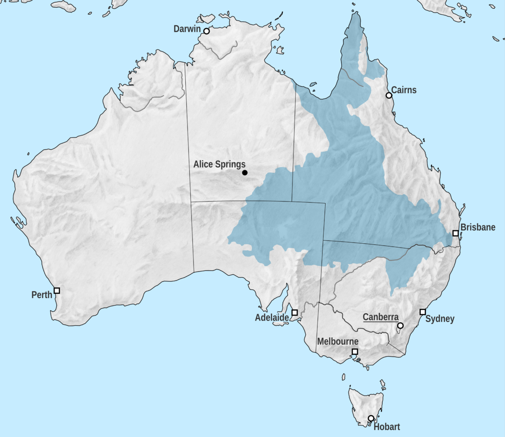
In many parts of Queensland, underground reservoirs (or aquifers) are the only reliable source of water. Across much of the state’s arid interior, human settlement and agricultural activities would be virtually impossible without water from the Great Artesian Basin — an enormous sequence of aquifers that underlies much of the eastern half of the country. Closer to the surface, there are numerous alluvial aquifer systems — the most significant being the alluvium of the Condamine River in the Darling Downs — which support regional towns and intensive irrigation districts.
Over the past century, many groundwater systems in Queensland have effectively been ‘mined’ as water has been taken at a rate faster than it is naturally replenished. Drastic reductions in water use from these systems have been (and are still being) enacted to return water extraction to within sustainable limits.
However, determining what these limits are is no trivial task. The workings of groundwater systems are largely hidden from view, and the only way to develop a picture of them is to drill holes in the ground and piece together the observations taken at each one. I remember a groundwater engineer in the department likening this process to punching holes into a book and reconstructing the plot by studying the confetti. That analogy might be a slight exaggeration, but it does illustrate why every hole drilled, and every bit of data collected, is so precious. We can really only guess at how a groundwater system works, and sometimes the data from a single hole will make all the difference between a good guess and a bad one.
The Groundwater Database and the open data revolution
To be of any use to anyone, all of this precious groundwater data needs to be collated and kept somewhere safe. The Queensland Government’s repository for this information is called the Groundwater Database. For just about every bore ever drilled in the state, the Groundwater Database contains information about when, where, and how deep the bore was drilled, as well as observations of things like water levels and water chemistry. I’ve heard that the database also contains a lot of rubbish, but nevertheless it is the accepted point of truth for groundwater information in Queensland.
My roles in the department never required me to actually use the Groundwater Database: that was left to the experts. The closest I ever got to it was in trying to negotiate the public release of another database that contained data derived from it. Despite none of that data being confidential, getting it released was an exercise in bureaucratic absurdity that went on for several weeks. This all unfolded in mid-2012. At that time, there were rumours that an Open Data Revolution was looming; but from where I stood, its arrival seemed a long way off.
Yet by the time I left the public service in March 2013 (or perhaps it was afterwards — that period was a blur to me even as it happened), the revolution had already come. The Queensland Government established an online data portal where anyone could download datasets that previously were available only after applying for a licence and paying a fee. All kinds of data, from flood imagery to financial statements, can now be downloaded freely from data.qld.gov.au — even the Groundwater Database! Better still, you don’t have do download a lot of this data to see it: you can explore it directly in Google Earth via the excellent Queensland Globe. Whatever this government has done wrong in the last two years, they have certainly done this much right.
Since I never needed to use the Groundwater Database while I was in government, you might wonder why I need it now. The answer is that I don’t, but it did present an opportunity that I couldn’t resist. Having recently learned how to make animated maps using the GIS software ArcMap, I wanted to see what a movie of the Groundwater Database would look like. If you ignore all of the information in the database about water levels, pumping rates, chemical constituents — basically all of the useful stuff — what you have left is a large series of points in space and time. These points have all been seen before by just about anyone who has used the database. But as far as I know (and I could be wrong about this), no-one has bothered to turn them into a movie.
Bores – the movie!
So here it is: 144 years of groundwater development, featuring 124,000 bores, 2 compressed into 72 seconds. 3 For the best viewing experience, I strongly recommend that you view the video in full-screen mode and in high-definition (the high-definition mode should kick in automatically after opening to full-screen, but if it doesn’t, then just select the ‘1080p’ option accessible via the cog icon just beneath the video). And don’t bother checking your speakers, because this movie is silent.
You could watch this video dozens of times (and I know some people who probably will) and still see new things. But a few notable features should be apparent even in the first viewing. For example, notice how in the first 50 years, the majority of bores accumulate within an arc running through the interior of the state. By 1920, this arc has resolved unmistakably into the outline of the Great Artesian Basin (discussed earlier). Meanwhile, a smaller, denser cluster of bores has started to appear just south-east of Dalby (which also happens to be where the very first bores appear in 1870). By 1950, this cluster covers the whole of the Condamine Alluvium (which I will examine more closely below).
In the first half of the animation, you also might have noticed that many of the bores appear in half-second pulses rather than in a continuous stream. This is an artifact of record-keeping rather than a reflection of reality. I suspect that the construction dates for these bores are estimates made long after the fact, and the dates were set to the 1st of January in whatever year was chosen. As the recorded dates become more precise, the animation becomes more fluid.
From the 1920s onwards, more small clusters of bores begin to emerge, including over the alluviums of Callide Creek (south-west of Gladstone) and the Pioneer River (north-west of Hervey Bay). By the 1950s, there are borefields around the coastal centres of Mackay, Townsville and Cairns. Nothing very surprising happens thereafter until about the year 2000, when there is a sudden flourish of activity across the eastern part of the state. This flourish must be the signature of the Millennium Drought, which affected Queensland (and indeed all of Australia) from 1995 to 2009. As rivers and dams dried up, it appears that people began installing groundwater bores even in places where none had been established before.
The big shift
The previous animation shows a cumulative view of bore development. Every bore remains visible indefinitely, regardless of whether it has been abandoned, replaced or upgraded. The bores gradually crowd each other out, and it becomes harder to distinguish new bores from old ones.
Instead of letting the bores accumulate, we can view them through a moving window of time, such as the three-year window used in the video below. This view shows more vividly how bore construction activity shifts over the years.
Particularly striking is the shift in the 1960s from the Great Artesian Basin to the alluvial systems in the eastern and coastal parts of the state. Also worth watching for is the Millennium Drought, which appears as a wave of activity that begins in about 2003 and dies down again in the final moments of the animation.
The Condamine and the South East
Even with the activity confined to a three-year window, the bores in areas such as the Condamine Alluvium are so densely packed in the previous animation that it is hard to see what is going on. The two videos below provide a more detailed view of the Condamine Alluvium and the surrounding region. As before, the first video shows the gradual accumulation of bores, while the second shows a moving three-year window.
The action in these videos is pretty slow at first, but by the 1930s you can see bores concentrating in the southern part of the Condamine floodplain. In the 1940s and 1950s, this development spreads north before kicking into overdrive in the 1960s. To the east, on the other side of the range, a series of short bands appear in the Lockyer Valley in the 1950s, followed in the 1960s by similar ladder-like patterns in the valleys of Warill Creek (south of Ipswich) and the Logan and Albert rivers (south of Brisbane). My guess is that these bores were installed to assess the future potential of these groundwater systems rather than to access and use the water. Interestingly, of these three systems, only the Lockyer Valley gets developed any further — that is, until just about everywhere gets developed during the Millennium Drought.
Going deeper
Having animated the spread of groundwater bores across the land surface, I wanted to visualise some aspect of their existence beneath the surface as well. The most obvious property to choose is how deep the bores have been drilled.
Drilling holes in the ground costs money, so typically a bore will be drilled only as deep as is needed to reach a good water source. If this water source is an alluvial aquifer, the bore might only need to be as little as 10m deep. If the water source is a sandstone aquifer in the Great Artesian Basin, then the bore will need to be much deeper.
The Groundwater Database records several different depth measurements, including measurements relating to water levels, bore casing and rock strata. Even the separate components of a bore’s casing are recorded separately, and these may be added to over time as the bore is deepened. I wanted just one measurement for every bore, so I filtered out everything except the deepest bore casing measurement recorded at the time a bore was constructed. 4 This still leaves more than 100,000 records.
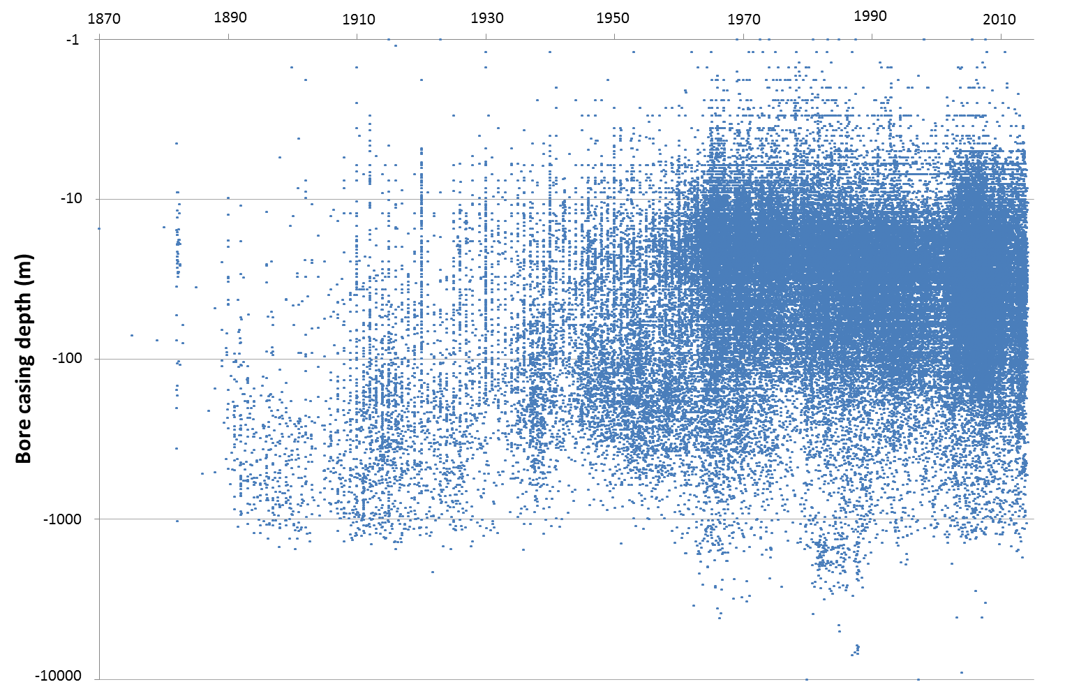
The usual way to summarise this amount of data would be with some key statistics such as the median and maximum depth for each year. But rather than abstracting the data, I wanted to see its inherent richness and complexity. As with the animated maps, I plotted the data in its raw form so as to let the eye perform its own analysis. In the graph below, time is represented on the horizontal axis and depth is measured on the vertical axis (with depth increasing as you move down the axis). Each dot on the graph marks the depth and approximate construction date of a bore.

Let’s look at the maximum depths first. By the 1890s, bore depths of around 1,500m are already common, and very few bores exceed this depth for several decades afterwards. Between about 1930 and 1960, there are few bores drilled deeper than 500m. Then suddenly in the 1960s, bores between 2,000m and 4,000m deep start appearing. Perhaps a new drilling technology became available at this time, or a particularly deep and good water source was discovered (someone out there must know!). In the 1980s, a small number of bores reach depths of 7,000m and beyond (I excluded some deeper bores for the sake of presentation). I suspect that these were drilled for research purposes rather than to recover water.
The graph above suggests that in all except the early decades, the majority of bores have been less than 500m deep. This observation backs up something that we saw in the animations: that is, a shift in bore construction activity away from the Great Artesian Basin towards the shallower alluvial systems nearer to the coast. Unfortunately, the shallow bores on this graph are packed so densely that we can’t see how they are distributed. To see this finer level of detail, I plotted the same data as before except with a logarithmic scale on the vertical axis.
Notice how the values on the vertical axis increase at each step by a factor of 10 rather than a constant amount. This allows the graph to squeeze in all of the data (including the bores at 10,000m) while still showing the distribution of the shallow bores. The explosion of shallow bore development beginning in the 1960s now stands out even more clearly. The majority of these shallow bores are between 10m and 100m deep, though it looks to me like they get gradually deeper (perhaps due to falling water levels) until about 2003, when there is a profusion of bores shallower than 10m, presumably in response to the Millennium Drought.
This graph also shows something else that we saw in the animations. Across the left-hand part of the graph, bores of varying depths stack into perfect vertical lines at regular intervals. The most obvious lines appear every 10 years, but in some places you can see them recurring annually as well. These lines correspond with the pulses in the early parts of the animations. They are the result of bores without precise construction dates being lumped together on the first day of a given year — or, we can see here, the first year of a given decade.
Seen yet another way – in 3D
If you are even slightly impressed by my modest visualisations of the Groundwater Database, then this should blow you away. The 3D Water Atlas project, which is being undertaken by researchers at the University of Queensland, has developed a Google Earth-style portal for visualising groundwater chemistry data in the Surat Basin, a geological sequence that forms part of the Great Artesian Basin. The atlas draws on data from the Groundwater Database as well as some other sources. As you can see in the video below, the results are very cool. I can’t imagine a better way to visualise and explore groundwater data!
In a similar vein is the Groundwater Visualisation Software developed by researchers at QUT. This software has been used to create some fantastic visualisations of aquifer systems including the Condamine Valley and the Lockyer Valley, both of which featured in the discussion earlier.
What’s new?
In one sense, I have presented nothing new here. Every one of the dots that you see in the animations and the graphs has been seen before, and I haven’t revealed any new facts about them — indeed, I ignored all but the most basic information available in the Groundwater Database. But in another sense, I think these products do convey knowledge that could not be seen any other way, or at least not with the same efficiency. Within the space of 72 seconds, these animations convey the pace and dynamics of 144 years of groundwater development history, from long-term and state-wide trends to fleeting local events.
I have no doubt that there are groundwater gurus and DNR veterans out there who know all about these trends and events already, having poured over the data for years or witnessed the developments first-hand. But for the rest of us, I’d like to think that these animations make that hard-earned knowledge more accessible. Not that the videos can convey this knowledge on their own: the context for their interpretation must come from those people who truly know what they are looking at. The real value of these animations will be realised when they are paired with a richer, more authoritative narrative than what I have provided here.
And perhaps the experts can learn something from these animations as well, in addition to seeing more vividly things that they already know. This is something that I am genuinely curious about. So whether you are a groundwater guru or not, I would love to hear your feedback on what (if anything) you have gained from seeing these videos.
Finally, I’d be interested to hear if there are any particular stories and events in Queensland’s groundwater history, besides the ones that I have alluded to, that could be usefully explored using these methods. It is relatively easy for me to make new versions of these videos that focus on particular times and places. I am not making any promises, but if someone makes a good suggestion, I just might be compelled to make some more movies.
Notes:
- The department wasn’t actually called this in all the time it was there, but for the sake of simplicity, that is what I am calling it here! ↩
- There are more than 148,000 bores registered in the Groundwater Database, many of them are missing information about their construction date and/or location, or the information that they do have is suspicious (unless someone in the department has a time machine). My attempt to filter out these records left a total of 123,979 bores. ↩
- In case you are wondering, the video was generated from fortnightly timesteps and encoded at 20 frames per second. ↩
- This measurement is the depth from the ground surface; it does not account for the elevation of the ground. ↩
Hi Angus
very very nice little piece of work. and well annotated and observant.