What we talk about when we talk about the lockdown
Back in January, I wrote a lengthy, data-driven meditation on the merits of my relocation from Brisbane to Melbourne. My concern at that time was the changing climate. Australia had been torched and scarred by months of bushfires, and I was feeling pretty good about escaping Brisbane’s worsening heat for Melbourne’s occasionally manic but mostly mild climatic regime.
But by gosh do I wish I was back in Brisbane now, and not just because Melbourne’s winter can be dreary. While Brisbanites are currently soaking up as much of their famed sunshine as they like, whether on the beach or in the courtyard of their favourite pub, Melburnians are confined to their homes, allowed out of the house for just an hour a day. During that hour, we are unable to venture more than 5km from our homes or to come within 1.5 meters of each other, leaving little else to do but walk the deserted streets and despair at all of the shuttered bars, restaurants and stores. All in the name of containing yet another existential threat that we can’t even see.
Of course, just because we can’t see the coronavirus doesn’t mean we can’t talk about it. Indeed, one unfortunate consequence of the ‘Stage 4’ lockdown 1 that’s been in place in Melbourne since the 2nd of August is that there is little else to talk about. We distract ourselves from talking about how bad things are by talking instead about how things got so bad in the first place. On days when our tireless premier (who at the time of writing has delivered a press conference every day for 50 days running) announces a fall in case numbers, we dare to talk about when things might not be so bad any more.

This post is anything but an attempt to escape this orbit of endless Covid-talk. Quite the opposite. In this post, I’m not just going to talk about the lockdown. I’m going to talk about what we talk about when we talk about the lockdown.
What Twitter is and isn’t
Well, not ‘we’, exactly — at least not if you take that word to refer to society at large. In this post I’m only talking about what is said on Twitter, which not even remotely the same thing. Only a small portion of the general population actually has a Twitter account, 2 and of those people who do, many (like me) use it mainly to see what other people are doing and saying rather than to share their own thoughts. Of those who do actively engage, many do so in bad faith, whether to harass other users or to push a hyperpartisan political agenda. Even worse, some accounts aren’t even people, but are instead automated ‘bots’ programmed to amplify hashtags or hyperlinks that would otherwise be ignored.
Given these caveats, a reasonable question to ask is why we should care about what happens on Twitter at all. One answer is that as niche and dysfunctional as Twitter is, it does intersect with and influence public discourse more broadly. To start with, it is teeming with the journalists and commentators who make and shape the news. It’s also a channel through which public figures from popstars to presidents bypass the usual gatekeepers entirely and broadcast messages directly to their followers. Conversely, Twitter provides a way for ordinary folk to challenge or expose privileged and powerful actors, fairly or otherwise. For various reasons, then, Twitter is a worthy object of study, as long as we don’t take it to be anything other than what it is.
Twitter also happens to be a very convenient platform to study. With the right software, it is relatively easy — and completely legal — to obtain thousands of tweets with accompanying metadata in a tabular format. With some patience (or paid access), you can amass a collection of hundreds of thousands, or even millions of tweets about a given topic.
The challenge: marrying up content with structure and dynamics
The hard part about working with Twitter data is therefore not obtaining it, but making sense of it. To be sure, there is no shortage of ways to go about doing this. For example, the field of network science, which was well established even before Twitter arrived, offers concepts and techniques for interpreting the structures and relationships that emerge from the interactions between twitter users as they mention, retweet (that is, quote) or converse with one another. With network analysis tools like Gephi, VOSON or (if you have an appetite for code) igrpah, you can probe these structures both visually and mathematically to do things such as identify communities of related users or determine which users are most influential in the discussion of a certain topic.
Less conceptually difficult to study than network structures are events and trends over time. For example, by plotting the number of tweets posted each day that contain a given hashtag or keyword, you can gauge the reach of a news story or marketing campaign. Or you might identify new growth markets by analysing long-term increases in the discussion of certain topics, as Twitter itself has done.
Then there is the content to consider: that is, the specifics of what users actually say inside their parcels of 240 characters or less. This is simultaneously the easiest and hardest aspect of Twitter data to get a handle on: easy because anyone can read 240 characters, but hard because no-one can meaningfully read and digest hundreds of thousands or tens of millions of these literary morsels, at least not without going mad in the process. There are two practical ways around this challenge: either read a small (and hopefully representative) sample of the full set of tweets; or reduce the complete set of texts to statistical summaries in the form of of keyword lists, topic models or sentiment scores. Ideally, you would do a bit of both.
In other words, there are ways to answer just about any well-formulated question about Twitter data. The methods and concepts are there: it’s just a matter of finding and applying the right ones with patience and rigour. But patience is a scarce resource, and rigour is expensive. Both should be conserved where possible and deployed only as needed.
One task that tends to demand more patience than I feel it deserves, and where I would happily sacrifice some rigour to save on time, is that of getting an overall impression of ‘what’s happening’ in a temporally distributed or structurally complex collection of texts, whether from Twitter or another source such as news coverage or another social media platform. As mentioned above, it’s easy enough to plot the number of tweets over time, or to visualise a network of interactions, or to summarise the keywords or topics. But seeing how the textual content varies over time or across network structures usually requires additional processing or cross-referencing of the data. For example, you might identify a peak in activity from a plot of tweets over time, then query the original dataset to browse tweets from that time period. A plot of topics (of the kind derived from LDA or a similar technique) over time might provide a useful halfway measure, but in my experience, you still spend a lot of time hunting down examples of tweets or documents that exemplify the topic and period of interest.
For this process to be really efficient, there needs to be a direct link between the temporal or structural representation of the data and the textual content in both its summary and raw forms. It all needs to be packaged together into a single, seamless product.
I have not yet come across an analytical tool that matches this description, at least not in the way that I want it to. That’s not to say that such a tool doesn’t exist, as my search to find one has not been exhaustive. But in any case, I took it upon myself to start building one. Heck, I had to find something to do while in lockdown. So in the remainder of this post, I am going to take the opportunity to road-test the analytical workflow that I have developed to visually analyse the content of Twitter data in tandem with either its network structure or its temporal dynamics.
I’m going to do this by using the workflow to examine how Twitter responded to the announcement and enforcement of Melbourne’s Stage 4 lockdown. I’ll say more about the technical details of the workflow later on, but will note here that I built it almost entirely in Knime, an open-source, graphically based analytics platform that I have written about extensively before. For a few operations, most notably to produce the final outputs, I also called upon R, in particular the Plotly and visNetwork packages.
I want to stress here that the main purpose of analyses that follow is to demonstrate the workflow rather than to uncover any deep insights about response to the lockdown measures. That said, I’ve done my best to tease out some interesting observations from the data, since this, after all, is what the workflow is supposed to enable.
Note also that while the workflow I am roadtesting here has been tailored to Twitter data, it could be adapted to other purposes. In particular, the method for seeing content as well as dynamics over time would be equally applicable to news or other temporally distributed texts.
The data
The dataset that I will analyse here contains a little over 20,000 tweets posted between the 1st and 10th of August 2020 that include the terms Melbourne AND (stage 4 OR lockdown). I obtained these using Knime’s own Twitter API Connector and Twitter Search nodes, running the query about once per day between the 3rd and 17th of August.
This dataset does not necessarily include all of the matching tweets created in this period, since the free tier of the Twitter API typically only returns a sample of all matching tweets each time you call it. However, judging from the declining number of new tweets retrieved each successive day, I suspect that the dataset is close to complete.
One sense in that the dataset is certainly not complete is that it does not include tweets that discussed the lockdown without explicitly using the terms Melbourne, lockdown or Stage 4. This limits the empirical conclusions that can be drawn from the analyses, since there could be significant chunks of the discussion that the dataset does not include. The dataset is more than sufficient, however, to test the workflow.
Seeing content over time
Figure 1 shows the volume of tweets over time about the Melboune lockdown between the 1st and 10th of August. The tweets are counted in 2-hour timesteps. Without knowing anything specific about the content of the tweets or who is posting them, we can already start to tell a story here. Something sent Twitter into a tizz very suddenly on the afternoon of Sunday the 2nd of August. After spiking, activity returned to an elevated level that evening, and decreased steadily over the next 24 hours. Then, beginning on the morning of Tuesday the 4th of August, activity pulsed in a daily cycle, with the peak diminishing each day after Wednesday the 5th of August.
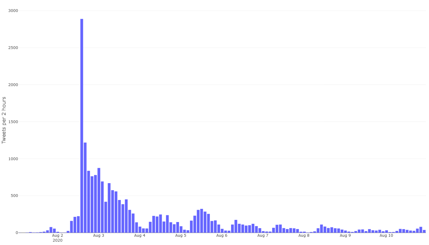
There’s no mystery around the huge spike on the Sunday afternoon. This was when Victoria’s premier, Daniel Andrews, formally announced that Victoria would enter a ‘state of disaster’ and that Melbourne would enter Stage 4 restrictions from 6pm that night. The spike coincides with the premier’s press conference, which began at 2:30pm. We can guess, then, that the big spike is the immediate reaction to the announcement, while the heightened activity over the following 24 hours is something akin to the reverberation of this initial shockwave.
The usual practice at this point would be to inspect popular tweets from different points in time to construct a narrative about what tweets, topics or events drove each day’s activity. That can be done easily enough by querying the underlying data, but this task could be made easier still by incorporating aspects of the content into the graph itself.
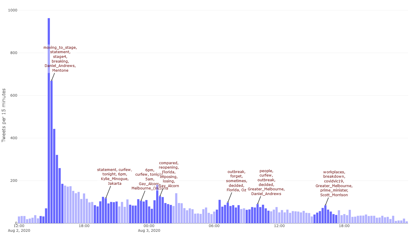
This is what I’ve done in Figure 2. The annotations in this graph list the most prominent words, names and user names appearing in the shaded ‘peak periods’ of activity. These annotations are generated automatically, based on term frequency statistics for the periods in question. The periods themselves are automatically detected using a simple formula that can be adjusted to catch sharper peaks or to cover larger windows of time. The result doesn’t always correspond with where a human might draw the boundaries, but the idea is that they are close enough to be useful for a first look. To read the annotations on the graph, you will probably need to click on it to see the larger image. But to see the full functionality of this graph, please open the interactive version.
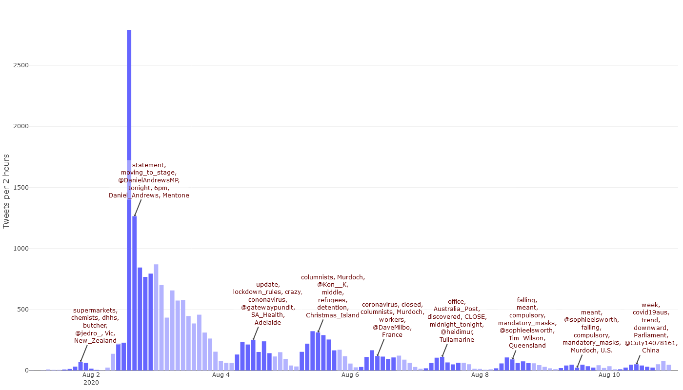
The annotations in Figure 3 can tell us a few things at a glance. First of all, we can see that the activity on Sunday afternoon was indeed focussed on Daniel Andrews’ announcement about Melbourne moving to stage 4 restrictions at 6pm that night. We can also see some unsurprising and thus easily interpreted terms emerging in the subsequent days, such as those referencing mandatory mask wearing and a downward trend in case numbers. The top terms on the 7th of August seem to relate mostly to the closure of post offices. There are also some terms whose relevance to the lockdown is not immediately apparent. On the 5th of August, for example, the discussion appears to be about refugees and Murdoch columnists.
What do refugees and Murdoch columnists have to do with the lockdown? We can’t know without seeing these terms in their original context. The interactive version of this chart makes seeing this context very easy: just click on a term, and you will be taken to the most popular tweet in the relevant period that uses it. For example, clicking on the word statement in the first peak period takes us to the tweet posted by Dan Andrews that contains his formal statement about the restrictions:
Statement on Melbourne moving to Stage 4 restrictions: pic.twitter.com/mFu1Kr1NO0
— Dan Andrews (@DanielAndrewsMP) August 2, 2020
Similarly, the word columnists over the 5th of August reveals this popular tweet by the journalist, Dave Milner:
Murdoch columnists are coronavirus superspreaders and should be closed under Melbourne’s Stage 4 restrictionshttps://t.co/I6ilxxtjFo
— David Milner (@DaveMilbo) August 5, 2020
Meanwhile, the word refugees links back to this tweet by Kon Karapanagiotidis:
It’s an act of naked depravity that Morrison Gov is apparently considering sending refugees detained in Melbourne to Christmas Island detention centre in the middle of stage 4 restrictions rather than release them safely into the community. The level of cruelty is unconscionable
— Kon Karapanagiotidis (@Kon__K) August 4, 2020
The annotations in Figure 2 are useful for understanding what’s happening during periods of high activity, but what if we are interested in moments outside these periods, or in specific timesteps within the peaks? The interactive chart caters to this need as well. Hovering the cursor over any individual timestep will bring up a box showing detailed information about the tweets in that timestep, as per the example below.
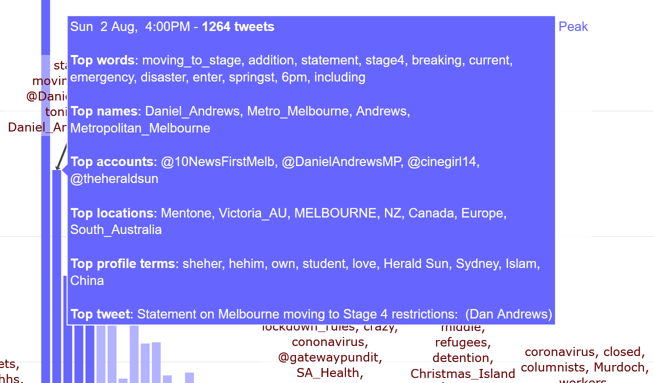
In a perfect would, this box would mirror the functionality of the annotations, and we would be able to click on any given term to see how it was used in context. Alas, Plotly (the R package that I used to generate the graph) does not yet offer a way to make these boxes ‘sticky’ so that you can click on their contents. Apparently this functionality is in the pipeline, so let’s hope it arrives soon. But for those of you dying to know what Kylie Minogue has to do with the lockdown, here is the relevant tweet:
Important to note that the Stage 4 restrictions in Melbourne do not prevent any of you from drinking a beer in the shower while dancing to Kylie Minogue's 2002 smash hit single Love At First Sight. If anything, it's encouraged.
— Cam Tyeson (@camtyeson) August 2, 2020
A closer look at Monday
One shortcoming of the graph in Figure 3 is that it did not include an annotation for any part of Monday the 3rd of August. This is because the peak-detection criteria that I used did not match any sequence of timesteps in this period. While we could fiddle with those criteria to force a spike to appear, we also have the option of simply examining this period on its own. This is what you see in Figure 4, which shows the activity from midday on Sunday to 11:59pm on Monday night. Each timestep is 15 minutes long. As before, you’re best to view the interactive version if you really want to explore it.
One thing we can see in Figure 4 is that people on Twitter kept talking about the lockdown well into the night after the Sunday afternoon press conference. After receding from the initial spike, activity remained steady from around 7:30pm until after 3am, and spiked again just before 1am. Were Aussie tweeps really staying up all night just to vent their misery or anger over the new rules? Some might have been, but most of this late night activity looks to have come from overseas. If you hover over the timesteps in the final hours of August 2, you’ll notice an increasing number of terms and locations relating to the United States and Europe, especially in the top profile terms (these come from the descriptions that users give to their own profiles). This shift is also evident in the annotation for the spike just after midnight, which includes Florida in addition to the account of Paul Krugman, a prominent American economist. Clicking on either of those two terms opens up this tweet (which also appears in many of the timestep pop-ups):
And Australia is imposing a full lockdown in Melbourne to stop this outbreak in its tracks; Florida, which is losing 180 people a day compared with Australia's 8, won't even require face masks and is reopening schools 4/
— Paul Krugman (@paulkrugman) August 2, 2020
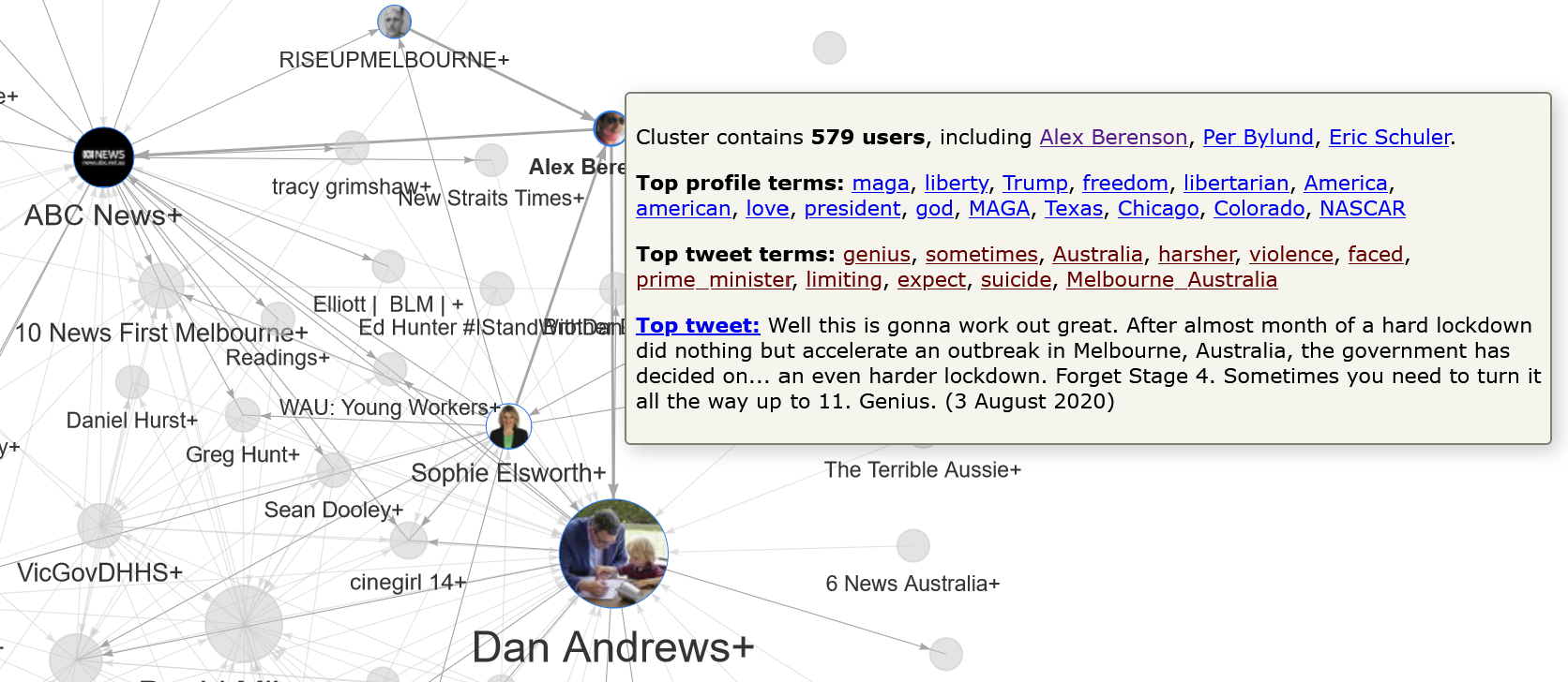
The timestep summaries from Figure 4 show that this tweet remained popular until 6:30am the next morning, when another US-based tweet took over, this time from the author and Covid-19 contrarian, Alex Berenson:
Well this is gonna work out great. After almost month of a hard lockdown did nothing but accelerate an outbreak in Melbourne, Australia, the government has decided on… an even harder lockdown. Forget Stage 4. Sometimes you need to turn it all the way up to 11. Genius. pic.twitter.com/ywWOD0UAKu
— Alex Berenson (@AlexBerenson) August 2, 2020
This remained the most popular lockdown-related tweet until business hours resumed in Australia, but it continued to be retweeted well into the day, as did Paul Krugman’s tweet. The last notable event in this time period is the bump in activity at around 4:15pm on Monday, which is when the prime minister, Scott Morrison, announced a pandemic leave payment for Victorians who had to self-isolate without access to sick leave.
The response to the press conference
Before moving on to a different visualisation, let’s see if we can learn a little bit more about what happened during the premier’s press conference on Sunday afternoon. Figure 5 shows the period from 2:30pm, which is when the press conference started, to 3:30pm, by which time I think (but am not sure) that the conference had concluded. Each timestep is a minute long. You can watch the first 27 minutes of the press conference on Youtube.
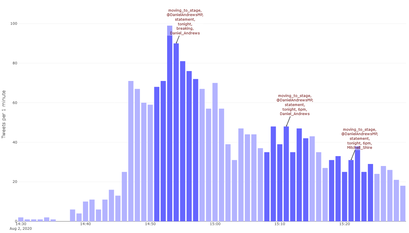
Although the press conference started at 2:30pm, few tweets about the lockdown appeared until eight minutes in. By watching the video, we can see that this was the point at which Dan Andrews finished announcing the new restrictions on movement in the Melbourne metropolitan area and turned his attention to new restrictions in regional Victoria. By hovering over the timesteps of the interactive graph, we can see that the activity at this point commenced with this tweet by 10 News First Melbourne (who in this case seem to have lived up to their name):
#BREAKING: From 6pm tonight, Melbourne will move to Stage 4 restrictions, including an 8pm to 5am curfew.
Victoria will enter a State of Disaster, in addition to its current State of Emergency. #COVID19Vic #springst #Stage4 pic.twitter.com/fxj0v7wVcb
— 10 News First Melbourne (@10NewsFirstMelb) August 2, 2020
This remained the most popular tweet in the dataset until 2:46pm, which is when things really started to take off. That was the moment when Dan Andrews gave a final recap of the announcements, and his office released the tweet I reproduced earlier containing his formal statement about the new restrictions. That tweet remained the most popular in the dataset for the remainder of the period shown in Figure 5, except where it was topped on a few occasions by the tweet from 10 News.
It’s important to remember that this dataset does not represent all Twitter activity that occured in response to the Stage 4 announcement, as it only includes tweets containing the words lockdown or stage 4 in addition to Melbourne. Many tweets may have referred to the same subject matter without using those specific terms. But to the extent that the dataset is reflective of the broader response, it tells a somewhat reassuring story. First of all, 10 News waited until the premier had finished announcing the Melbourne restrictions before releasing its tweet, even though there might have been a temptation to jump the gun in order be first. Secondly, the tweet that eventually stole the show and got the most attention was the one posted by the premier himself, showing that there is an appetite among many Twitter users for authoritative information.
Seeing content across the network
The foregoing examples show that with the use of automated annotations and interactive tool-tips, it is indeed possible to bring the dynamic and qualitative aspects of Twitter data a little closer together. But what about the relationships between tweet content and the network structures defined by user interactions?
A standard way to represent twitter data is as a network of users connected to one another by way of mentions and retweets. The network for the Melbourne lockdown dataset (minus those users who are connected to only one other user, or who are part of clusters not connected to the main network) is shown below.
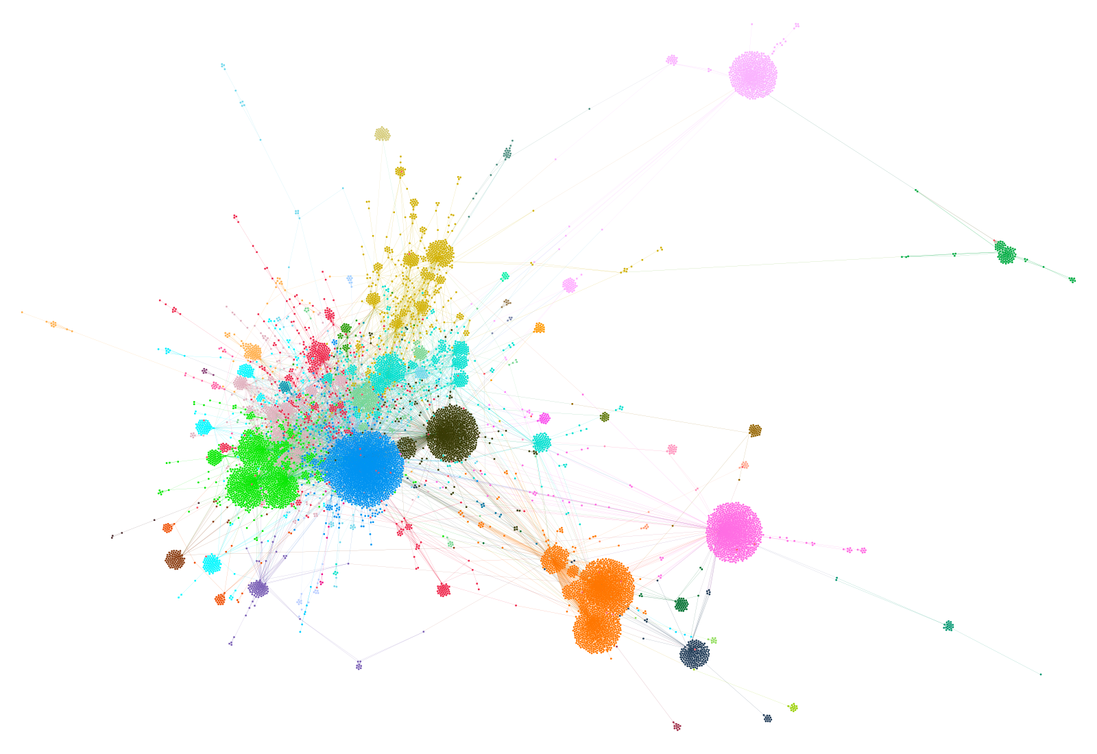
Despite containing more than 12,000 users, this network’s structure is not overwhelmingly complex. This is because most of the users are clustered into tight hubs around frequently mentioned users. The big blue hub in the centre, for example, consists mainly of users who retweeted Daniel Andrews, while the isolated pink hub at the top-right is a community of users who retweeted Alex Berenson. The more interesting structures in the network are those defined by the connections between these hubs. Towards the bottom of the network, for example, is a cluster of several hubs (coloured orange) that are tightly connected to one another. So interconnected are these hubs that they have been grouped together (by a community detection algorithm) into a single community that is structurally distinct from the rest of the network. By looking at the colours in the network, you can see several other clusters of hubs that have been similarly grouped.
Grouping the users into hubs and clusters in this way is a useful way to see the structure of the network, but it ultimately doesn’t help us much unless we learn what defines and differentiates the clusters. Who are their members? What topics have they tweeted about? What interests or attributes do they share? A visual inspection of the network can tell you the names of the users, but typically not much more. If we have the right data processing skills, we could assemble some statistics for each cluster, such as the number of members and who among them is most influential. We might even go further and identify the most prominent terms used by the users in each cluster. To be really useful, though, this information needs to be available on-demand from within the network visualisation.
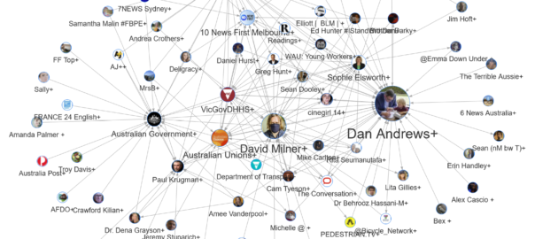
This is the vision that I’ve tried to realise in the output presented below. In essence, what I’ve done is create a simplified version of the network by collapsing each of the clusters into single nodes, and enriched the result with interactive annotations that are automatically generated based on the data within each cluster. The interactive, web-based output is possible thanks to the wonderful R package, visNetwork. Figure 7 shows a static image of the output, but to play along at home, please use the interactive version.
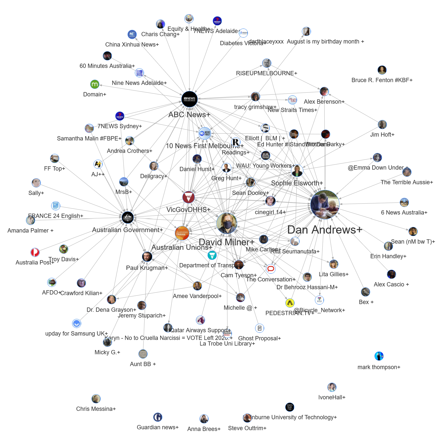
Don’t let the labels mislead you: the nodes in this network are not individual accounts, but clusters of multiple connected users. The size of each node reflects the total number of mentions or retweets from users in other clusters. The pictures and labels reflect the most frequently mentioned user in each cluster. In many cases, this user is the only prominent member of the cluster, and the remaining members are there only because they retweeted the main user. In some cases, however, a cluster may contain several prominent users. For example, the Australian Government+ cluster includes Helen Sullivan and SBS News, both of which were mentioned or retweeted by many other users. As it happens, the hubs around these users are those visible in the orange cluster discussed previously in Figure 6.
Obviously we can’t see the full membership of each cluster from within in this condensed version of the network. However, by hovering over any node in the interactive version, you can see the top three members, along with other summary information:
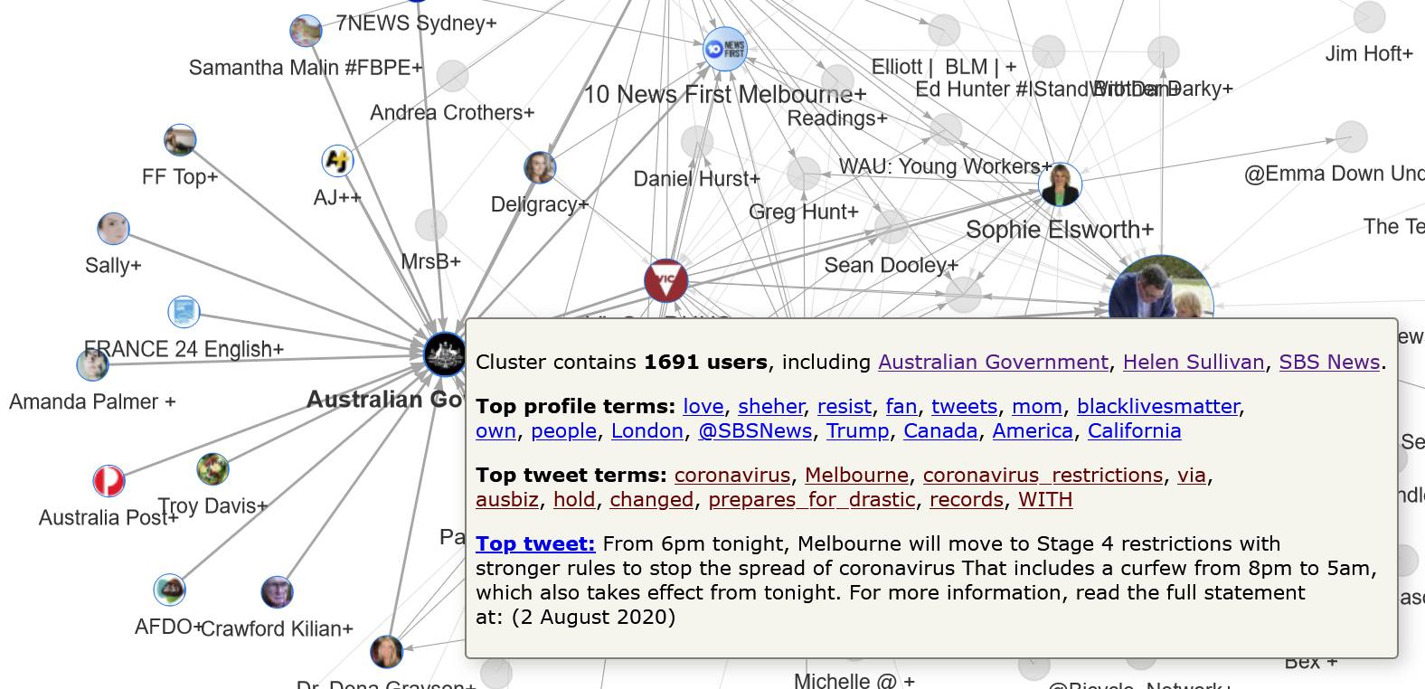
In this case, we can see that Helen Sullivan and SBS News are among 1,691 users in the cluster. We can also see from the top profile terms (extracted from the user profiles) that users in this cluster probably come from around the world, and especially the United States. The namesakes of the clusters connected to the Australian Government+ cluster, which include a French news service, the American singer Amanda Palmer, and the American economist Paul Krugman, confirm the international reach of this cluster.
Clicking on any of these top profile terms will open up the most popular account (as measured by mentions in the dataset) whose description contains the term. Similarly, clicking on a top tweet term will open the most popular tweet from the cluster that contains the term. Lastly, the pop-up box shows the text of the top tweet in the cluster, which in nearly all cases is authored by the namesake of the cluster.
This interactive visualisation therefore enables us to see the high-level structure of the network while also having immediate access to information about the membership and content of each cluster. Furthermore, the hyperlinked terms and account names take us straight to representative examples of actual tweets and profile pages.
With this information at hand, what can we learn about the discussion of Melbourne’s lockdown on Twitter? Given what we learned in the earlier analysis of activity over time, we should not be surprised to see Dan Andrews at the centre of the most mentioned cluster in the network. This cluster is also the largest, containing 2,183 users. Also unsurprising is the centrality of 10 News First Melbourne, given that they were the first news organisation in the dataset to break the news about the Stage 4 restrictions. Other characters we’ve encountered already include Paul Krugman, Alex Berenson and David Milner. Now, however, we can see how these characters (or rather, the communities of users that mentioned them) are connected, and who else they connect to.
We’ve already noted that the Australian Government+ cluster includes and connects to a lot of accounts from overseas. By contrast, the top terms and connections of the Dan Andrews+ cluster suggest more local connections, which might help to explain why these two clusters are located at opposite ends of the network. One overseas user who is connected to the Dan Andrews cluster is Alex Berenson. As mentioned earlier, Berenson has been described as a Covid contrarian for his skeptical views about the risks posed by Covid-19 and the merits of lockdowns such as the one in Melbourne. The pop-up information about the Alex Berenson+ cluster (shown below) suggests that most of his followers are of a conservative or libertarian persuasion — very much the opposite of the lockdown policies that Dan Andrews has introduced.
Why, then, are these two clusters connected at all? The interactive visualisation cannot answer that question definitively, but can provide some relevant information. If you hover over any link in the network, a pop-up will appear with information about the number of connections, the direction of those connections, and a link to the tweet that links the most prominent connected users. In this instance, we learn that there are just two connections between these clusters, both of which involve mentions or retweets from users in the Alex Berenson cluster:
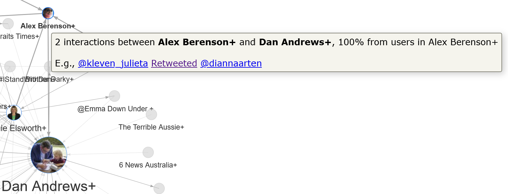
The example tweet that links the clusters turns out to be from an Australian BlackLivesMatter supporter posting an article from the Guardian — hardly what we expected to find in the Alex Berenson cluster, but a good reminder that we should not expect these clusters to be uniform in their membership.
Some of the other connections to the Alex Berenson cluster are less surprising. RISEUPMELBOURNE is a local chapter of the conservative, Christian, patriotic lobby group, Rise Up Australia, while Jim Hoft is the founder of the Gateway Pundit, a highly conservative online American media outlet. Also worth mentioning is the cluster centred around Sophie Elsworth, a columnist for the conservative, Murdoch-owned News Corp. This cluster, which also includes The Herald Sun and 7 News, is connected to all three of the abovementioned conservative clusters. While the physical centrality of the Sophie Elsworth+ cluster indicates that it is probably mainstream in nature, it clearly serves as a bridge between the Australian mainstream and some more extreme right-wing networks.
There’s a lot more that could be unpacked in this network, but the above examples are sufficient to illustrate the functionality of the visualisation. As with the earlier analysis, it’s also important to remember that this network is not a complete representation of users tweeting about the Melbourne lockdown, as it does not include users who might have discussed the lockdown without using the three keywords that defined my search query.
The workflow
The interactive charts and network presented in this post were rendered in R using the Plotly and VisNetwork packages. But the information fed to those packages is the result of some rather complex pre-processing, nearly all of which took place in Knime (the only exception being the use of the iGraph package in R to identify the network clusters). All components of the workflow, including both R scripts and Knime nodes, are incorporated into a single Knime workflow thanks to Knime’s R integration capability. I principle, it could all be converted into a single R package (or better still, with a shiny interface). This would be an interesting project, but a major one.
In some previous blog posts, I have shared the Knime workflows (with embedded R scripts) that I used to produce the visualisations. I’d love to share the Kode (my word for the equivalent of code in a Knime workflow) for the visualisations that you see above, but it’s not quite in a state fit for sharing, and I’ve learned from previous experience that the final step of getting a workflow to that point can be very time-consuming. And since I’m doing this all in my own time (which, admittedly, I have rather a lot of right now), I’m not about to make any promises about if and when this workflow will be ready to share.
That said, I may well find motivation in the interest of others, if any such interest is forthcoming. So please do drop me a line if you think you could use what you see here.
Notes:
- To date, we’ve been from Stage 3 back to Stage 2, and then up again to Stage 3 before ratcheting up to Stage 4. Hopefully we’ll be back to Stage 3 in a few weeks. We keep using that word, but I don’t think it means what we think it means. If I lapse into calling it ‘Level 4’ instead, that’s why. ↩
- According to this report, there were just over 5 million Australian Twitter users in January 2020 (many of which would be organisations rather than individuals), compared with 16 million active Facebook users. ↩
A solid blog post that contains an enormous amount of research. This network analysis approach using topic analysis of social media data and temporal ‘hooks’ to a broader reality is pretty cool . And I like the way in which you critique your quantitative data (and the tools) using qualitative ranking of its contextual significance. A well-rounded, educational, and reasoned approach. Ace!